Why Has Lucky Imaging Not Been Possible before?

The principal difficulty with this method is the performance of the CCD cameras that are used at telescopes. CCD detectors are now very close to being theoretically perfect. They have nearly 100% quantum efficiency, superb imaging and cosmetic quality, are available in large areas (the biggest manufactured and sold commercially so far has 110 million pixels) and a very robust electrically and mechanically. Astronomers generally read out their cameras slowly (typically 30-500 kilohertz pixel rate) in order to minimise the readout noise, the noise that is added to every pixel, irrespective of the light level within it, because of the amplifier on the CCD output. If the CCD is read out quickly enough to be useful for Lucky Imaging (5-35MHz pixel rate) the readout noise is very much higher, typically 100 electrons per pixel per frame read. As an example, with Lucky Imaging we may select 4,000 images out of a total run of 40,000. If the readout noise was as high as 100 electrons per pixel per frame we would find that our summed image has a noise floor that is 64 times higher (square root of 4,000) than the single frame read noise. This would be 6400 electrons per pixel in background noise alone. This will have a dramatic effect on our overall sensitivity. A star image is detected over perhaps 10 pixels and therefore it would need to have something of the order of 300,000 electrons (detected photons) to get significantly above this background noise level.

What has happened recently is that an entirely new output structure (known as low light level CCDs or L3CCDs) has been developed for CCDs by E2V Technologies (Chelmsford, UK). Similar technology electron-multiplying CCDs (EMCCDs) have been developed by Texas Instruments (Japan). Both work by extending the output register with an additional section that is clocked with much higher voltages than usual so as to give a noiseless electron multiplication stage before the output amplifier. This signal amplification stage effectively reduces the readout noise of the on-chip amplifier by the gain factor of this multiplication register which may be set as high as many thousands. A single frame read out at high speed has essentially no readout noise with this technology. It is possible to build cameras that can see each and every individual photon detected by the CCD chip. The effect of this is that our limiting sensitivity is dramatically increased to perhaps only 30-100 detected photons from the reference star per frame, a factor of over 3000 on the above example. Lucky Imaging is therefore only possible because of this new technology which we have used in our experiments and observations. For more details of how EMCCDs work in click here.

How Do We Measure Image Quality and Select the Best Images?

In order to assess the quality of individual short exposure images we need to have some reference object in the field of view with known characteristics so that we can compare what we see in each picture with what we would expect ideally in the absence of any phase fluctuations. For ground-ground imaging this will be some sharpness criteria while for astronomical imaging we use an unresolved reference star in the field of view. In practice we compare the ratio of the peak brightness of the reference star in each image with that which we would get in the absence of phase fluctuations. This is called the Strehl ratio. We use the Strehl ratio measured on each frame to order the images in a sequence by quality. The best images are then aligned with one another before adding into the total. If we restrict our sum to the very best images we clearly get the very best resolution but we also degrade the signal-to-noise because we will be using so little of the light coming into the telescope (if, for example, we discard 99% of the images). We can increase the signal-to-noise at the expense of resolution if we include a larger fraction of the images. The effect of this is shown in the images below. Plots are for star 10 arcsec from reference star, 12 Hz frame rate and:

1% selection, 0.13 arcsec FWHM

3% selection, 0.14 arcsec FWHM

10% selection, 0.16 arcsec FWHM

30% selection, 0.18 arcsec FWHM

The Limits Imposed by Atmospheric Turbulence

Elementary diffraction theory (see, for example, Born & Wolf, Principles of Optics (2nd Edition), 1964, Pergamon Press) shows that the resolution of a telescope in the absence of any atmospheric fluctuations is given by 1.22 (λ/D) where λ is the wavelength used, and D is the diameter of the telescope. This gives us the resolution we should expect at different wavelengths with telescopes of different sizes.

Pass Band:	1m diameter	2.5m diameter	4m diameter	7.5m diameter	10m diameter	40m diameter
B, 450nm	0.11 arcsec	0.044 arcsec	0.028 arcsec	0.017 arcsec	0.011 arcsec	0.0028 arcsec
V, 550nm	0.14 arcsec	0.056 arcsec	0.035 arcsec	0.019 arcsec	0.014 arcsec	0.0035 arcsec
R, 650nm	0.16 arcsec	0.064 arcsec	0.04 arcsec	0.021 arcsec	0.016 arcsec	0.004 arcsec
I, 850nm	0.21 arcsec	0.084 arcsec	0.052 arcsec	0.028 arcsec	0.021 arcsec	0.0052 arcsec
J, 1.2 microns	0.30 arcsec	0.12 arcsec	0.075 arcsec	0.04 arcsec	0.03 arcsec	0.0075 arcsec
H, 1.6 microns	0.40 arcsec	0.16 arcsec	0.10 arcsec	0.053 arcsec	0.04 arcsec	0.010 arcsec
K, 2.2 microns	0.55 arcsec	0.22 arcsec	0.14 arcsec	0.073 arcsec	0.055 arcsec	0.014 arcsec

In practice even the best Observatory sites find that the resolution they achieve with conventional astronomical imaging is only about 0.5 arc seconds at visible wavelengths. Short exposure images of bright stars show that the shape and resolution obtained varies dramatically from image to image. Fried (1978) discussed the method of using Lucky Exposures in detail and some experimental results were obtained in the 1980s both in astronomical and ground-ground imaging. The results were interesting but hopelessly limited by the then very poor performance of the camera systems available at the time.  Lucky imaging principles have been used really quite extensively by the amateur astronomy community who have been able to take very high quality images of bright objects such as Mars and the other planets. There is more information about Amateur Lucky Imaging here.

Turbulence in the Atmosphere.

Theoretical models of turbulence in the atmosphere were developed in the middle of the 20th-century particularly by Tatarski (1961), and were developed from some much earlier studies of turbulence by Kolmogorov (1941). Their models assume that turbulent power is initially generated on the largest scales and that dissipative forces cause the turbulent power to be transferred to smaller and smaller scales, eventually being dissipated on scales much smaller than those with which we are concerned here. These models make a good number of predictions about the characteristic length and timescales of the turbulence and in particular about the power spectrum of the fluctuations that will be found.

In this model, refractive index variations in the atmosphere produce phase fluctuations (amplitude fluctuations are much less significant) in the wavefront entering the telescope. The phase fluctuations are assumed to have a Gaussian random distribution and the model may be characterised by a single parameter, r₀, which correspond roughly to the diameter of the telescope whose resolution is beginning to be significantly affected by atmospheric phase fluctuations. At good observatory sites typical values for r₀ are 20-40 centimetres in the I-band (850nm). Because the phase fluctuations are random there is always a chance that the phase across a single cell of diameter r₀ will be much smaller than average. There is a smaller chance that the phase across several cells will be smaller than average. The bigger the diameter of the telescope the larger the number of cells across its area. The chance that most of the cells have a much smaller than average phase fluctuations across them clearly goes down with telescope diameter and eventually becomes so unlikely as to be negligible. However at intermediate diameters the probability of the phase fluctuations being much smaller than average is still significant and if those images can be selected and accumulated while those that are poorer than some level are discarded them clearly the image resolution will be significantly improved.  This is the basis of the Lucky Imaging method.

Measurements of Atmospheric Turbulence

It is not practical to measure the instantaneous three-dimensional turbulent structure in the atmosphere. What we are able to measure by the effects of the turbulence on star images or generally on the wavefront coming into a telescope. A lot of information can be derived simply by taking pictures of the pupil of the telescope as can be seen below:

And to see a movie (2Mbytes, mpeg format) click here

Kolmogorov Models May Be Too Simplistic

The power spectrum that one obtains from these studies does indeed agree rather well with the Kolmogorov turbulence predictions but we have to be clear that these experiments do not demonstrate that the turbulence is therefore simply a Gaussian random process with a Kolmogorov power spectrum.  The atmosphere that we look through is very much a two-dimensional structure. The aspect ratio of the atmosphere over the Atlantic Ocean is very similar to the aspect ratio of an A4 sheet of photocopier paper . Sheets of air at slightly different temperatures and humidities slide over one another with turbulence being developed only where adjacent sheets touch. In some cases we should not expect full three-dimensional turbulence to be established, and we may find that power on one scale of turbulence may be transferred to larger scales (as happens with two-dimensional turbulence) as well as to smaller scales (as happens with three-dimensional turbulence). Even the most casual observation of cloud structures shows that really rather fine structures in clouds can persist for relatively long periods (perhaps an hour or more for structures only 1-2 metres across), something that should not be possible if the motions in the atmosphere were simply characterised by true three-dimensional turbulence. We also know from other studies which we have made on large telescopes where we were trying to track the development and evolution of turbulence that it is surprisingly common for what appeared to be jumps in the phase which move across the telescope aperture relatively quickly and will cause a complete loss of lock for an Adaptive Optics system.

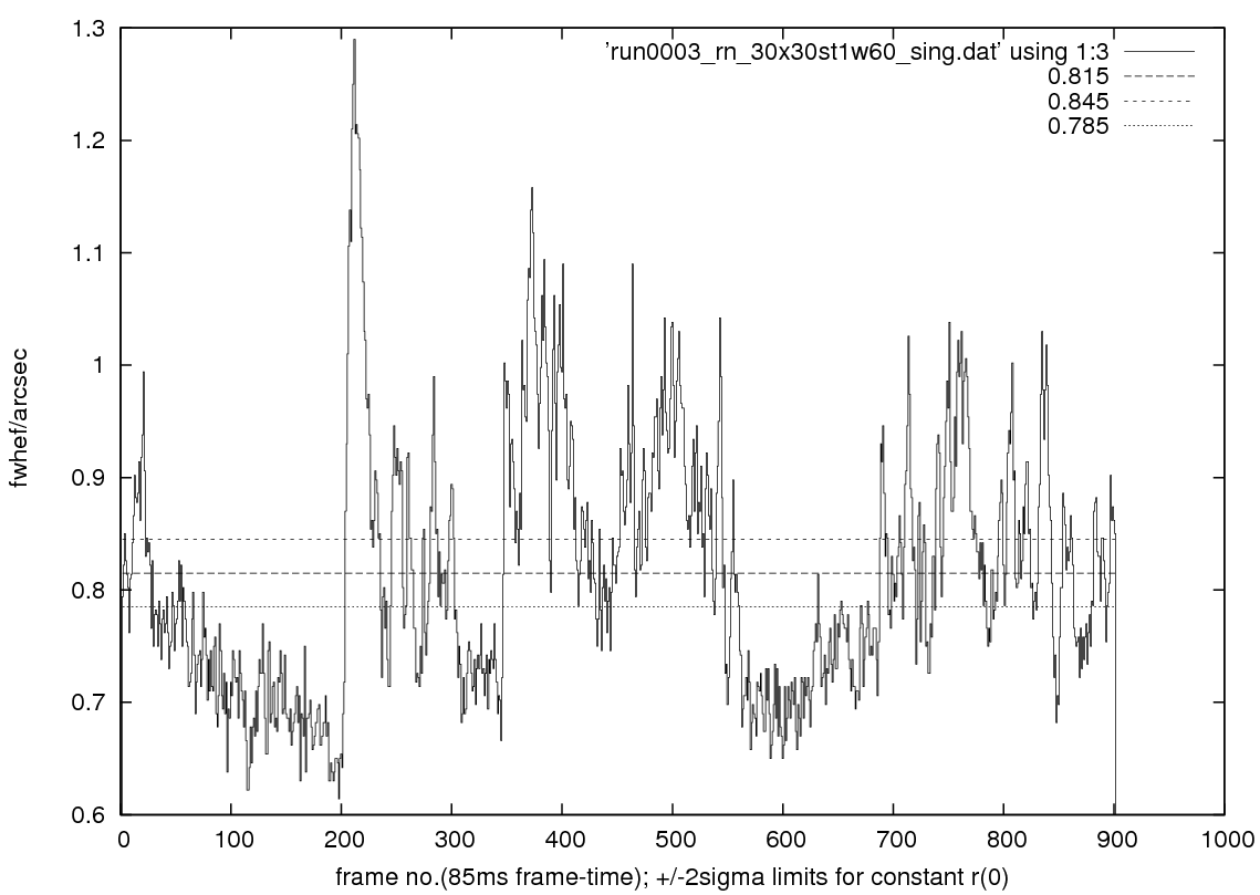
Figure: The variation in image profile width over a single 80 second long run, at 12 frames/sec.  Note the very rapid changes in seeing characteristics.  Adaptive Optics systems invariably assume that the phase errors are always free from discontinuities and so cannot follow such steps.

We see events which may or may not be related with Lucky Imaging where occasionally the image will split rapidly into two or more components, one of which fades as the other brightens. With Lucky Imaging we happily discard these frames, but with adaptive optics the system keeps trying to hold things together and ends up by adding in light which may indeed be less well imaged that if the Adaptive Optics system was simply not present.

The complexity of the Adaptive Optics system means that it will take many tens or hundreds of readout frames before it can stabilise and re-establish lock on the wavefront errors coming into the telescope. While this is happening poorly corrected or even positively mis-corrected image is continue to be accumulated on top of the existing integration.