All of the semester 05A WFCAM on-sky data is online in Cambridge in MEF format, including: the phase-II commissioning; Science Verification data; UKIDSS data; and the rest of the scheduled observations for PATT time, University of Hawaii time and Japanese time. Data from semester 05B has also been steadily arriving, roughly two weeks after taking the observations, and is ingested and verified in Cambridge typically within a few days of arrival.
There are occassional detector dropouts during observing which are either picked up during ingestion or during pipeline processing. Examples of this are detector #2 had "zero" data values for the latter quarter of the night of April 11th and the latter half of the night of June 18th. (This appears to be caused after an individual data acquisition PC crash; the subsequent reboot sometimes leaves the system in a null frame of mind). In 05A there were also occassional (1 in 10000) missing individual detector frames from other nights. Many of these "disappeared" during format conversion and transfer to tape. These issues have been followed up with JAC and where possible the missing files have been found, transferred and included in the online dataset. Several improvements to the data verification at the summit have been implemented to minimise the re-occurrence of similar problems and for 05B these missing frames are now at the level of less than 1 in 100000.
All of the raw data is available online through the WFCAM raw data archive centre in Cambridge (the UKIDSS data and all calibration frames are also being transferred from Cambridge to the ESO raw data archive). Access to the Cambridge archive is password protected. Registration is through the on-line interface. Note that although the data is stored using Rice Tile compression (see eg. Sabbey 2000 PASP 112 867) an uncompress on-the-fly option is available for retrieval - though we recommend transferring the compressed images due to the ~x 3 reduction in bandwidth required.
Each night is separately pipeline processed using master calibration twilight flats updated at least monthly; but, where possible, locally generated darks and sky-correction frames are created and used. After checking, the processed data products: images, confidence maps and catalogues, are automatically transferred to WFAU in Edinburgh for ingest in the WFCAM Science Archive using multi-threaded scp-like protocols with transfer speeds of around ~10Mbyte/s. To date some 25 Tbytes of raw WFCAM data are held in store (~8 Tbytes with Rice compression) with roughly 40 Tbytes of processed products created (~10 Tbytes with Rice compression).
The first pass processing for all of the semester 05A data was completed by the end of July and all the 05A data was preprocessed during August and September to include improvements to the pipeline made during CASU SV analysis. The real-time status of the data transfer from JAC and of the pipeline processing in Cambridge is automatically monitored and made available online together with other general WFCAM information.
The philosophy behind the data processing strategy is to minimise the use of on-sky science data to form "calibration" images for removing the instrumental signature. By doing this we also minimise the creation of data-related artefacts introduced in the image processing phase. To achieve this we have departed somewhat from the usual NIR processing strategies by, in particular, making extensive use of twilight flats, rather than dark-sky flats (which potentially can be corrupted by thermal glow, fringing, large objects and so on) and by attempting to decouple, insofar as is possible, sky estimation/correction from the science images.
The following processing steps are applied to all images, though in practice no linearity correction is currently required
Most of the sky correction is additive in nature and caused by illumination-dependent reset anomaly and pedestal offsets. Residual gradients introduced by the twilight flatfielding strategy are negligible across detectors and are well below the 1% level. The pedestal offsets can be quite large, typically +/-4% of sky (we know they are additive since there are no equivalent photometric systematics - see later). The more variable quadrant on detector #4 also stands out.
All the detectors show similar cross-talk patterns. The cross-talk artefacts are essentially time derivatives of saturated stars with either a doughnut appearance from heavily saturated regions (+/-128xm pixels either side, where m is the interleave factor mxm from microstepping eg. 1x1 2x2 3x3, plus progressively weaker secondaries further multiples on), or half-moon-like plus/minus images from only weakly saturated stars. Adjacent cross-talk images have features at ~1% of the differential flux of the source, dropping to ~0.2% and ~0.05% further out. Beyond three channels the effect is negligible. The following figure illustrates where cross-talk images are expected in detector X-Y space relative to the position of saturated objects for each quadrant (note that the orientation of the detectors on-sky also rotates by 90 degrees between each detector - see the commissioning report for an illustration of this). The cross-talk pattern rotates from quadrant to quadrant because the readout amplifier for each quadrant is on a different edge of the detector (denoted by the red lines).
The good news is these artefacts
are non-astronomical in appearance and do not "talk" across the detector
quadrant boundaries, or between detectors; the bad news is that they do not
generally jitter stack out.
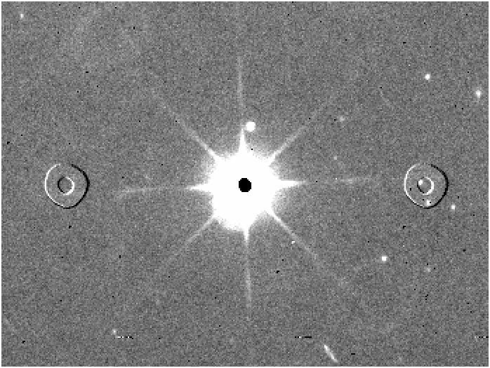
Some examples of cross-talk are shown below.
The first shows the cross-talk from a heavily saturated image, with an
alternative view of the saturated image to illustrate the cause of the problem
(ie. the cross-talk image is to first order the time derivative of the signal
in the saturated image channel along the readout direction.

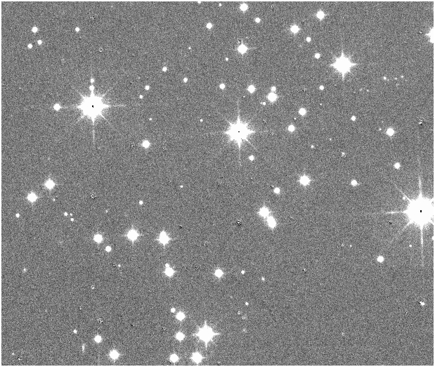
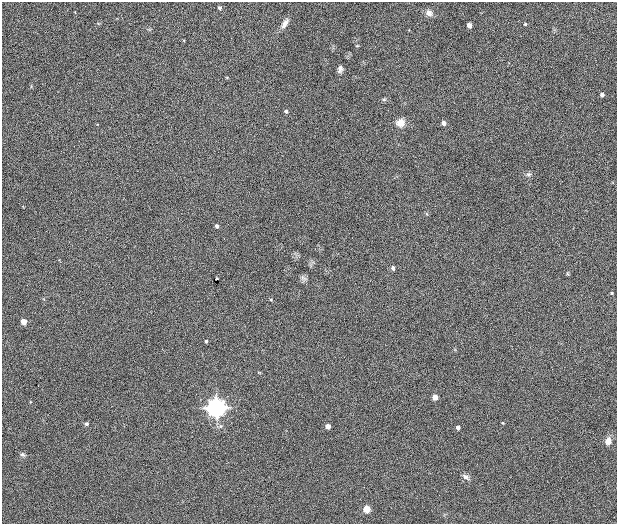
Significant cross-talk only appears to be generated by saturated images as is evident in the field of the open cluster shown below to illustrate the overall nature of the problem.
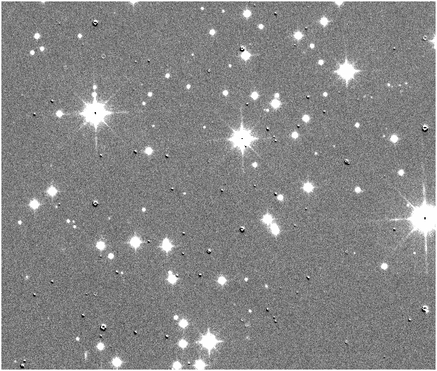
Athough this is stacked image and not strictly appropriate, the cross-talk removal software is sufficiently general that we show below the result of applying it to this image since the cross-talk artefacts stand out more clearly.
Illumination correction measures are ongoing via two methods: one based on the mesostep sequences and the other, highly promising method, based on stacking multi-frame 2MASS residuals as a function of spatial location. Initial results from this latter approach are extrmeley promising, ie. although residual spatial systematics are present, they are measurable and appear to generally be at the +/- ~few % level. An excellent example of this mapping is provided by stacking all the residuals from the WFCAM calibration photometry for data taken on photometric nights in June which were all processed using the same twilight flatfields.

The above plot shows the average spatial photometric residuals from a large number of different pointings taken during June 2005. (A correction for astrometric radial distortion is automatically applied during the 2MASS calibration amounting to up to ~1.5% at the outermost corners.) The average magnitude of the residuals in this case is less than 2% and is (probably) caused by a mixture of: gradients in the twilight sky - but this must be at a low level since flatfielded dark skies do not generally show significant gradients across detectors; scattered light in the flatfields - dark skies would also suffer from similar problems so cannot be used to correct it; significant spatial PSF variation, particularly earlier in semester 05A - monitoring using photometry from larger radius apertures shows this effect is present (and hence correctable) but at steadily decreasing level from April through to June (see the other examples of the spatial photometric residuals in the J-band for April and May and compare these with the residuals derived using a larger aperture - 4 arcsec diameter cf. to 2 arcsec - for April , May , June ).
Monitoring the spatial systematics in the photometry is still ongoing but one early conclusion is that it has negliglible effect on the overall derived zero-points which are a robust average of the data from all detectors for each calibrated pointing.
We have re-measured the overall colour equations with respect to the 2MASS system using the much broader colour spread of standards observed as part of the April SV data. This has still been done via visual inspection but the bigger colour range reduce the errors to ~0.025 for JHK and ~0.05 for Y and Z. Using 2MASS matches for the nights of 8-10 April inclusive gives the following ce's:
      Z_wfcam  =  J +  0.95*(J - H)   2MASS  [previously 0.9
      Y_wfcam  =  J +  0.50*(J - H)                      0.4
      J_wfcam  =  J - 0.075*(J - H)                     -0.1
      H_wfcam  =  H + 0.040*(J - H) -0.04               +0.15
      K_wfcam  =  K - 0.015*(J - K)                     -0.05]
these were used to calibrate the WFCAM instrumental magnitudes in the
2MASS photometric system. [Note that the old values above were used
for the first SV release from the WSA. The -0.04 constant offset for the
H-band is needed to bring the 2MASS H-band system onto the standard Vega
scale.] Further checks using all of semester 05A data and the first month
of 05B data demonstrate that these colour equations now only need very small
further adjustments (ie. the effects are at the < ~1% level).
With these new colour equations and a much better run of data we have rederived the system zero-points (corrected to unit airmass) for the main passbands. These are shown in the next table. Note also that in deriving these zero-points, all detectors have been gain-corrected to the average detector system
                                Z      Y      J      H      K
Overall zero-point  (count/s) 22.84  22.77  23.02  23.24  22.57
WFCAM                  (e-/s) 24.4   24.4   24.6   24.8   24.2
[using an average gain of 5.1 = 4.3 after correcting for intrapixel
capacitance]

UFTI                   (e-/s) ----   ----   24.5   24.7   24.2
This gives the following WFCAM sensitivity figures for 5s exposures, 0.6 arcsec seeing and a 2 arcsec diameter aperture. Aperture corrections to/from other data should assume a Moffat profile with beta=2, which gives a 0.15 magnitude aperture loss in this case (included in the computation).
                                Z      Y      J      H      K
5-sigma limiting mag  (5s)    19.6   19.0   18.4   17.8   17.1
                     (40s)    20.7   20.1   19.5   18.9   18.2

Sky (mag/sq arcsec)           18.0   17.0   15.6   14.0   13.4
Darks are routinely computed from the daily observations, by combining as many darks as are generally available (within reason) for each exposure time and readout mode. If a particular combination is not available the nearest suitable calibration dark frame from nearby nights is used instead. If this still doesn not produce all the required darks to process a night's data, a suitable cunning combination of closely related dark frames is created and used instead.
The single frame confidence maps are generated in conjunction with the twilight master flats. In principle sufficient (dawn) twilight flatfield frames to form master flats are taken once per week using a series of 9-point jitter sequence observations in Z,J,K and Y,H. It is impossible to get good flats in all broadband filters in any one night. Suitable individual 9-point jitter sequences (~5000-20000 counts/pixel ie. ~25000-100000e-/pixel) are dark-corrected and then scaled and robustly combined to form new master flats (if enough are availalbe these may be further combined to reduce the random photon error in the master flats even further). If available a pair of these flats at different counts levels (~factor 2) is then used to automatically locate the bad pixels and create the generic confidence map, one for each filter. Bad pixels are defined as those having properties significantly different from their local neighbourhood "average" in the individual master flats or in their ratio.
The majority of the sky correction stage is actually correcting crud on the field lens (glows and scatters external light). There is no measurable fringing present in any of the passbands in any of the filters. A series of sky correction frames are generated using a collection of grouped dark sky science frames (including photometric standard frames) taken at suitable [intervals throughout the night. The collection group has to satisfy a number of requirements to produce a viable sky frame, including: a minimum number of independent pointings (ie. separated by more than a specified distance); and not taken in special locations (eg. centred on bright NGC galaxies or in very crowded regions). The individual sky group components are combined by scaling to a common level. Sky correction then proceeds by scaling the chosen sky frame to the data and additively applying it, whilst maintaining the original overall average sky level. Typically ~5 sky correction frames are generated in each passband per night. The sky frame closest in temporal location to the target frame is used for the correction.
with the maximum level of the reset anomaly about a factor x10 less than it used to be, only reaching ~50 ADUs at the outer readout edges of the quadrants.
The curtaining problem remains at about +/-5 ADUs, and can be seen at low level in the darks. It is, however, best illustrated from the difference between two dark frames of the same type.
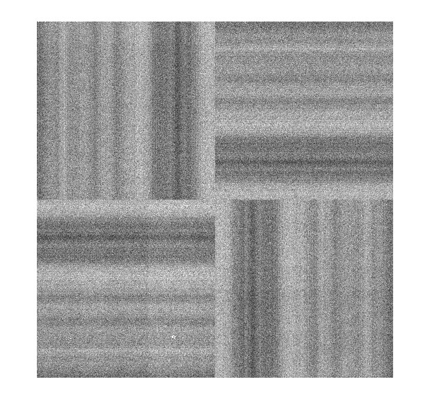
Decurtaining is now part of the pipeline reduction software, and is illustrated in the decurtained difference dark image below.
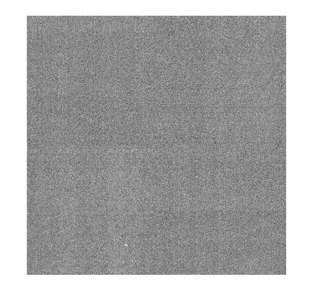
Not only does the decurtaining algorithm remove the curtaining problem it also is used to reduce the effect of residual reset anomaly on normal astronomical images (see later section). It works by robustly estimating two 1D 1024 additive correction functions making heavy use of iterative clipped medians and the 4-fold 90 degree quadrant symmetry of the detectors.
After decurtaining the difference between successive darks can also be used to estimate the global r/o noise from differences of assorted dark frames. Science frames are either being taken using CDS or NDR mode. A comparison of single exposure CDS darks and multiple read NDR darks are given in the table below (the numbers are taken from the earlier commissioning report which should be consulted for further details.
 difference image noise   frame               single frame noise

  #1  #2  #3  #4
  6.5 6.8 5.4 7.2       dark20_cds   av r/o noise  = 4.6   ADU
  6.5 6.2 6.6 6.0       dark5_cds                    4.5
  4.0 5.0 4.5 5.5       dark10_ndr                   3.4
There is no significant difference between the 5s and 20s CDS darks.
Note that in an ideal world m NDR frame reads gives approximately sqrt(m/3) improvement [not sqrt(m) because the resulting readouts are correlated] on r/o noise over normal CDS mode. In NDR mode the resulting output frame is computed internally in the DAS from the gradient of the flux increase for each pixel (ie. flux/s) and then normalised back to the total count for that exposure time.
The darks appear to be stable on timescales of a few days.
More recent measurements of the r/o noise and gain from the April 2005 SV data are given in the table below. The r/o noise was estimated from the difference between successive single exposure CDS 5s dark frames after running the decurtaining algorithm to remove systematic artefacts. Note that the average dark current is generally negligible and dominated by reset anomaly variations. The gain is the average of gains measured at 3 background levels 23k, 14k and 5k; the overall variation in measured gain was at the ~0.05 level with no clear trends with background.
   detector  dark current  r/o noise (ADU)   gain   r/o noise (e-)
     #1          -2.4          3.8           4.84       18.4
     #2           3.7          4.2           4.87       20.5
     #3          -9.0          4.2           5.80       24.4
     #4          49.1          4.4           5.17       22.7
Whilst doing these measurements of the gain from the dome flat sequences,
an estimate of the inter-pixel capacitance via a robust measure of
the noise covariance matrix was also made. This was remarkably consistent
from detector to detector and is summarised below:
                      0.00 0.04 0.00
                      0.04 1.00 0.04
                      0.00 0.04 0.00
plus much smaller coefficients in adjacent rows and columns further out.
A sum of the noise covariance matrix close to 0,0 gives a value of
1.20 which implies that the total reduction in directly measured noise
variance (ie. measured using a conventional method) is therefore also 1.20
(Parseval's Theorem and power spectrum <-- FT --> autocorrelation).
This therefore
predicts a ~20% overestimate of the gain, and hence a ~20% overestimate of
the QE coefficients. This apparently is as expected for the Rockwell
Hawaii-II devices.
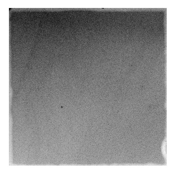
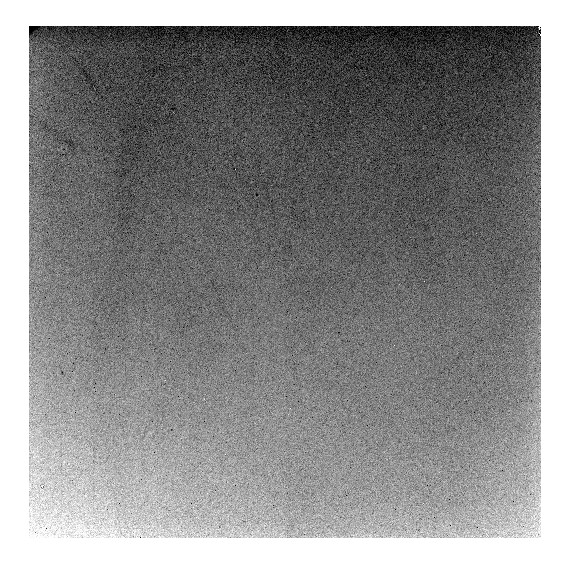
Twilight flats taken during the SV phase have been used to compute master flats for all the broadband filters ZYJHK. There is a surprising amount of large scale non-uniformity in the flatfield counts within detectors. Since the general characteristics of these variations can be seen across all filters the simplest interpretation is that these variations in level reflect genuine sensitivity variations across the detectors (this has been subsequently confirmed by examining the chisq values of residuals from PSF-fitting).
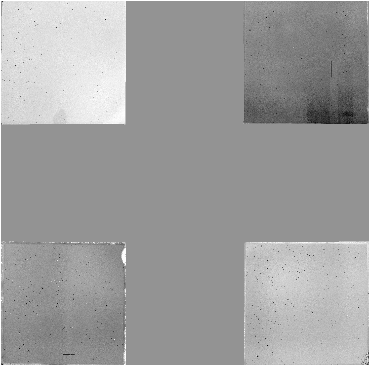
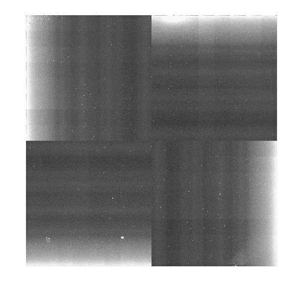
As an illustration all 4 detector H-band master flats for the period 7th-19th April are shown in mosaic overview in the following figure (N to top E to left).
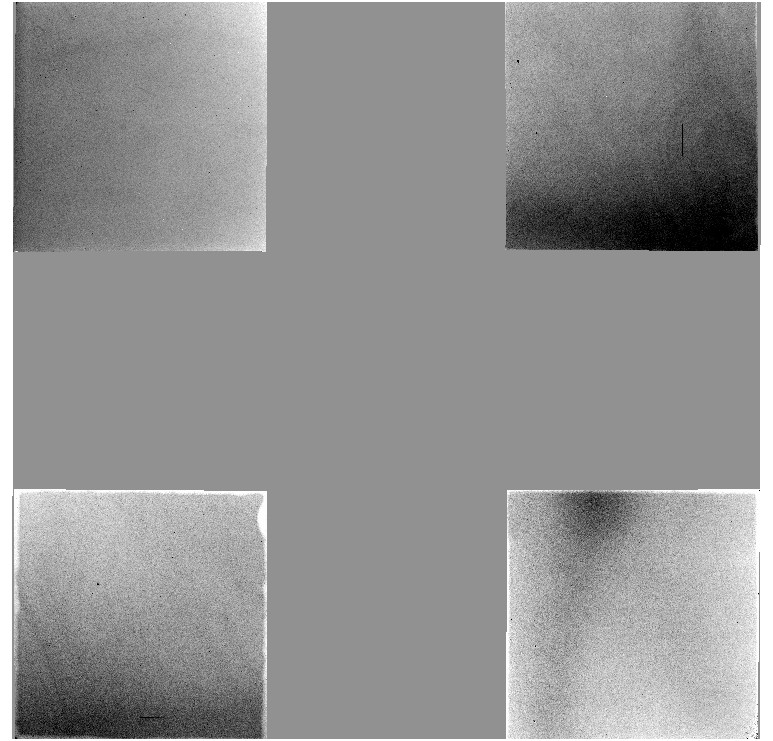
There is a large apparent sensitivity variation on all detectors, whereby the response seems to vary by up to a factor of 2, This in turn also causes problems for the generation of confidence maps, uniformity of surveys, and possibly also impacts on the calibration error budget.
This is quantified in the following series of histograms which show the recorded sky level normalised to the median level of all 4 detectors (ie. these are notionally the gain corrections)
although the "average" sensitivity is good there are significant regions on most detectors a factor of 2 worse, these are the darker regions in the figures below
these variations are also present in dark sky (ie. not caused by weird illumination gradients in twilight flats) as evinced by the flat background present in the flatfielded processed data before any sky correction phase. Also given the spatial distrubtion of the sensitivity gradients (see on-sky mosaic) they are unlikely to be vignetting either.
Detector#1
Detector#2
Detector#3
Detector#4
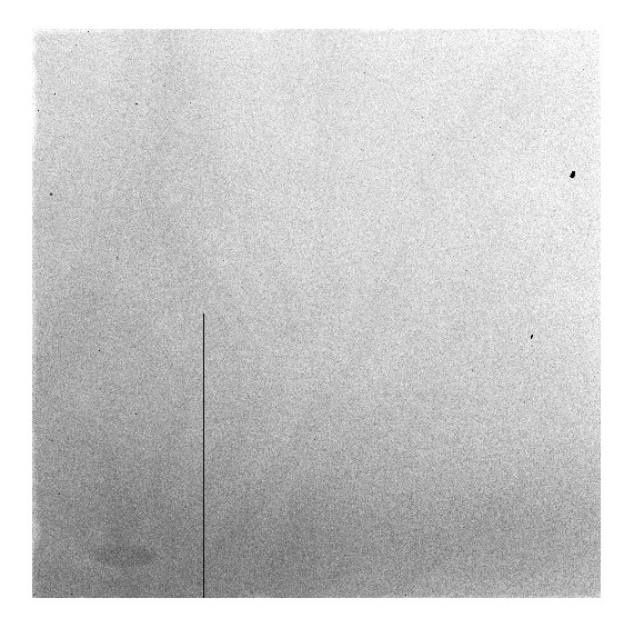

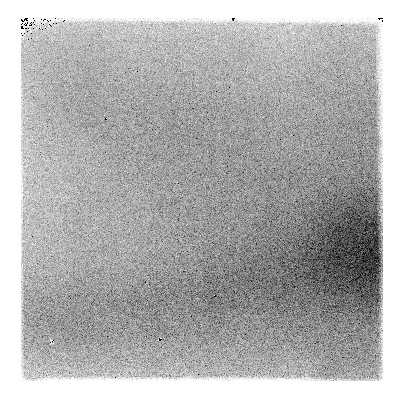
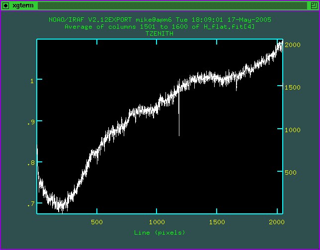
A slice through columns 1501 - 1600 for detector#4 is shown below to illustrate the dominant variation is a global gradient rather than rms noise.
In the sets of examples shown the following steps were taken:
1. Only frames passing sensible quality control criteria were used, ie.
seeing < 1.0 arcsec, average ellipticity < 0.2, reasonably photometric
night from visual inspection of the nightly photometry.
2. The object catalogues were matched detector by detector using a 2.5
arcsec search radius with an iterative 6 constant linear solution applied
to matched objects to improve the differential astrometry. Typical
differential astrometry averages much better than 100mas for the whole region.
3. Objects matching within 1.0 arcsec were considered reliable matches,
ie. the probability of a spurious mismatch is low even in such crowded
regions. Objects matching in the range 1.0 - 2.5 arcsec were flagged as
unreliable using the classification index.
4. The colour magnitude diagrams were constructed from all objects classified
as stellar (ie. cls = -1 or -2 in all bands). In addition, for the
colour-colour diagrams, objects were only plotted if their estimated
magnitude errors were < 0.1 mag in each passband.
5. For tiles and larger areas a unique object catalog was constructed by
searching for duplicate entries within 1 arcsec and retaining the entry
with the lowest magnitude error.
05A Science data examples
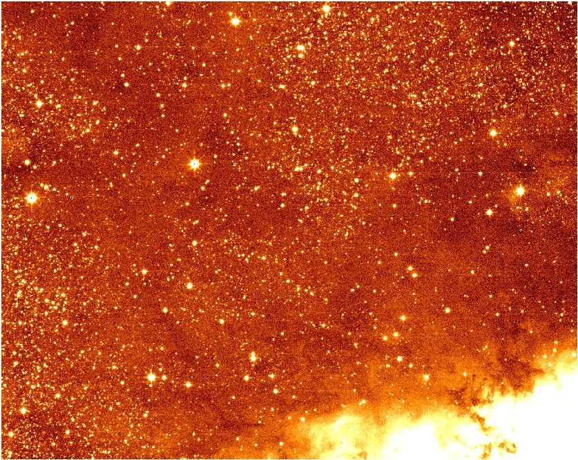
JHK photometry from M17 region
The example photometry diagrams come from data taken in June 2005 and
come from one detector covering the region
illustrated below. Note in particular the huge variation in redenning
across even this small region (14' x 14').

YJ photometry for IC4665
This example comes from catalogues from several tiles taken during April 2005
which when combined cover a total of 3 sq degrees centred on IC4665.
Photometry for a complete LAS tile
This example comes from LAS catalogues in Y,J,H,K from 4 separate pawprints
from SV data taken on 8th April 2005. These were combined to form a tile
covering 0.7 sq degrees on sky. Stellar-classified sources are shown as
black dots, non-stellar as red.

Mike Irwin (mike@ast.cam.ac.uk)
Last modified: Thu Jan 26 14:50:38 2006