The previous reports ([Evans 2004a], [Evans 2004b]) on PSF
fitting for the WFCAM project have mainly dealt with development of the
software and tests
on simulated data. Since then suitable observations have been carried out
with WFCAM and tests involving real data can be performed.
In [Evans 2004b] it was found that the PSF model that performed best was that
of the elliptical Moffat profile. However, it was stated that this was
probably due to the simulations using Moffat profiles to generate the images.
Tests on real WFCAM data (the UDS test data, see Section 6) showed that
a more detailed model was required. The one chosen was the adaptive kernel
method described in [Alard & Lupton 1998]. The details of the model used is
given in Appendix A.
A problem with the adaptive kernel model is that it is not as robust as the
elliptical Moffat profile model due to its larger number of parameters.
These problems are caused by contaminating images affecting the sampled PSF.
Current work is aimed at finding the balance between having enough images to
define the PSF adequately and remove the effects of contaminating images.
A number of modifications have recently been carried out to the PSF
measurement as described in [Evans 2004a] in order to make it more robust:
The Hanning filter has been modified so that the averaging is carried
out using medians rather than the usual mean. This is important in cases
where there are not many images and that the median averaging used in the
summation of the oversampled PSF has not eliminated any contaminating images
due to there only being one image contributing to a cell.
The fitting of the adaptive kernel model is carried out in two stages
with residuals larger than 4σ (Gaussian) rejected for the second fit.
The weighting that is used in the fit is inverse variance with the
variance having been measure during the process of applying the Hanning filter.
Future work: while the oversampled PSF is being built
up, only non-contaminated areas from each contributing PSF is used. This is
determined from the information contained in the catalogues.
Note that the sampling and the adaptive kernel fit are carried out using a
square aperture since this is more appropriate for the model being used
since a large part of it is not radially based.
Although much data has been taken with WFCAM, it is not entirely trivial to
find suitable data to measure the performance of all observing modes of the
camera. For the DXS and UDS surveys this can be done, but for the other
surveys it is not possible since repeat observations have not been carried
out. Many repeat observations are available from non-UKIDSS observations,
but these are taken in different observing modes.
The following comparison was carried out on stacked, interleaved data taken
in K on the same night. The seeing for these images was 0.8-0.9".
The observing parameters were: 2x2 interleaving,
Njitter=9, exposure time 5s, Nexp=2, thus giving a
total exposure time of 360s.
Using the same procedure as in the previous reports, since
3 repeat frames are available, it is possible to determine the
external astrometric and photometric errors for each frame. This assumes
that the errors are not correlated ie. they are independent.
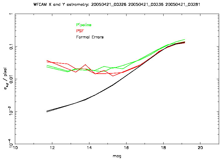
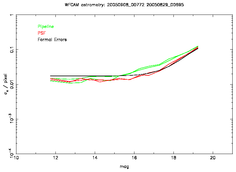
Figure 1: This plot shows the relative astrometric errors as a function of
magnitude for a single frame for the observations described in the text.
Also shown are the quoted formal errors for the PSF astrometry. Note that
the pixel scale shown is 0.4". Also, the formal errors in this plot
do not take into account the effects of atmospheric turbulence.
Figure 1 shows the results of the astrometric comparison. Over
most of the magnitude range PSF fitting produces slightly better astrometry
than the standard pipeline. In the mid-magnitude range the improvement is
almost by a factor of 2. At the bright end both the accuracy of the pipeline
and PSF astrometry reach a limit of 0.02 pixels (8 mas) for this particular
case. There is a hint that the PSF accuracy is slightly worse at the bright
end
A number of other comparisons were carried out with similar results.
The formal errors match the measured errors very well at the faint end, but
the measure accuracy reaches a limit at the bright end. This is the same
result as found in the second report ([Evans 2004b]). This limit is explained in
Section 6 of [Alard & Lupton 1998] and is caused by turbulence in the
atmosphere. For 1" seeing they quote
σd ~ 2(θ/rad)1/3(t/sec)-1/2arcsec
Using values of θ = 1000 pixels, 0.85" seeing (also using a
linear approximation) and 360s exposure, the predicted limit is 11 mas. This
formula also gives a limit comparable to that found for the INT data in the
second report. Using the various limits found from the comparisons carried out
an empirical scaling was determined to give the following relation:
This is now added in quadrature with the originally calculated formal errors
and is now what is quoted in the catalogue files for the PSF astrometric
errors. Tests were carried out on data with different total exposure times
to confirm that the above astrometric limit was correct.
These tests are for relative astrometry and involve using a simple
6-parameter plate solution to match the images from each detector. If a more
detailed plate solution were to be used, it might be possible to improve the
astrometry limit. For example, if each detector were split into 4 regions and a
plate solution applied to each region, then it is likely that the astrometric
limit would be improved by a factor of 21/3=1.26.
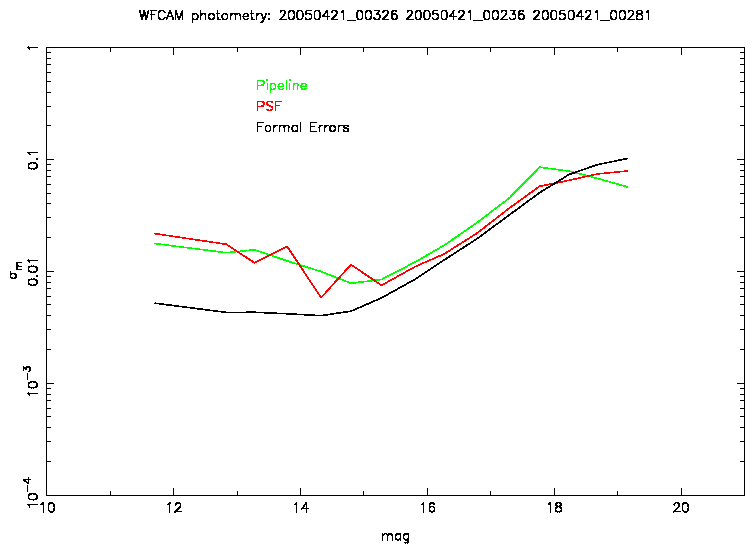
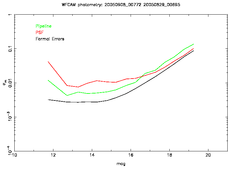
Figure 2: This plot shows the relative photometric errors as a function of
magnitude for a single frame for the observations described in the text.
Also shown are the quoted formal errors for the PSF photometry.
From the tests carried out with WFCAM data, not much difference is found
between the standard pipeline and PSF photometry (see Figure 2).
The formal errors are
close to the measured errors at the faint end, but are a factor 4 too small
at the bright end. As with the astrometry, this limitation could be linked
to atmospheric effects, but it is likely that other factors are involved. In
all cases checked, the errors increase at the bright end. This is possibly
due to saturation effects reducing the validity of the PSF used.
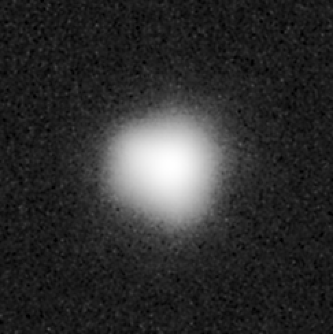
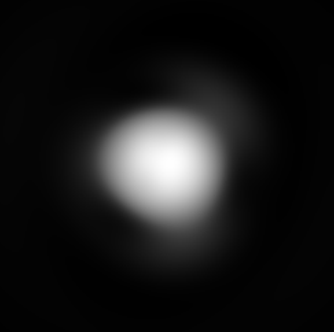
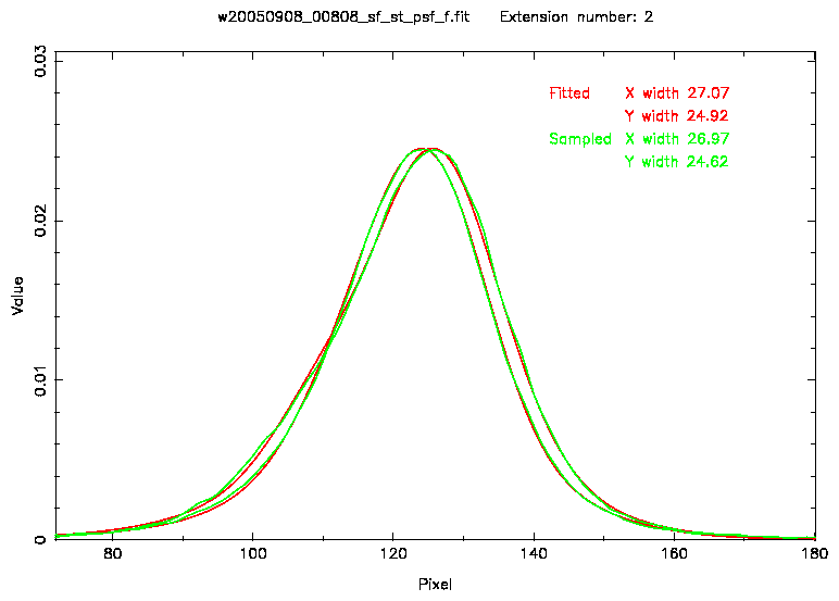
4 The shape of the PSF and its variation across the field
The following plots (Figures 3 and 4) show the
shape of the PSF from detector 3 for the stacked and interleaved (3x3) image
20050908_00808 (taken for the UDS microstepping test). The difference
between the sampled and fitted PSFs is small
and shows that the adaptive kernel model works well. This example shows more
structure than most of the PSFs measured.
Figure 3: This plot shows the sampled and fitted PSF from the stacked and
interleaved frame 20050908_00808.
Figure 4: This plot shows the X and Y slices through the middle of the
PSFs shown in Figure 3.
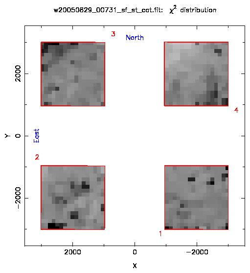
In order to see if the PSF is varying across the field of view the reduced
χ2 values are plotted as a function of position. These values are
derived from the χ2 values from the PSF fit and are divided by the
number of degrees of freedom. Figure 5 shows the variation for
frame 20050829_00731 which is also a stacked and interleaved (3x3) image.
Across the
field of view there is a small amount of variation of the reduced χ2,
indicating that the PSF might vary. The variation of the
reduced χ2 is generally between 0.95 and 1.05, except for detector 4
where it is between 0.90 and 1.10. It is known that detector 4 has problems
in one quadrant which will affect the sky estimation and this in turn the
PSF fit.
Figure 5: This plot shows the reduced χ2 values across the field of
view of the camera for the stacked and
interleaved frame 20050829_00731. Midtone grey corresponds to a value
of 1.0, white 0.7 and black 1.3
A Hanning filter (3�3 Bartlett filter) has been applied to the data.
The red outlines show the location of the 4 detectors.
Tests have been carried out on a number of whole nights (20050408 and 20050409)
to assess the performance and robustness of the PSF measuring programme.
In total, 485 PSFs were measured and only in one case did the PSF measuring
procedure fail. In many cases, odd shaped PSFs were measured, but on closer
inspection prove to be correct. These are usually caused by a failure in
the observing.
These tests took about 1.5 hours per night of observations to
carry out the PSF measuring and 2.5 hours for the PSF fitting. These tests
were carried out on one of the 2GHz AMD processors of apm3.
Some data was taken for the UDS survey to test microstepping. This data was
taken on 29 August and 8 September.
The seeing is similar for both nights (0.6"-0.7").
Sadly only 5 frames are available, so
only a limited test can be carried out. If this test were to be repeated
then the observations for each mode should be repeated at least 3 times
(preferably on the same night) and the total exposure time for each mode
should be broadly similar. A 1x1 test should also be carried out to show
that interleaving is required in the first place.
Note that the data for this test was not on the UDS field, so there
are no other repeats of these frames. The details of the frames are as
follows:
Nustep
Njit
Texp
Nexp
Total exposure
20050908_00772
2x2
9
5s
2
360s
20050908_00808
3x3
9
5s
1
405s
20050829_00695
2x2
9
5s
1
180s
20050829_00695
3x3
9
5s
1
405s
20050829_00695
3x3
9
5s
1
405s
Due to the limited data, the comparison carried out was a direct one scaled by
√2. This is reasonable due to the seeing being similar.
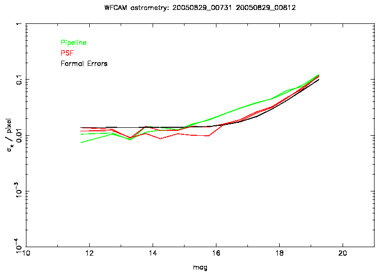
Figures 6 to 9 show the results from this
comparison. Again, note that by pixel the original uninterleaved pixel
=0.4" is meant. The astrometric formal errors shown in these plots
include the astrometric limit described in Section 3.
The slight complication in this test is that the 2x2 frames differ in their
exposure times by a factor 2.
A reasonable estimate to account for this is that the 2x2
plots need to be adjusted by 20% (ie. make them better) in order to get a
level playing field.
If you do this, there is next to no difference between the two operation
modes.
Figure 6: This plot shows the relative astrometric errors as a function of
magnitude for the 2x2 UDS test.
Note that the pixel scale shown is 0.4".
Figure 7: This plot shows the relative astrometric errors as a function of
magnitude for the 3x3 UDS test.
Note that the pixel scale shown is also 0.4".
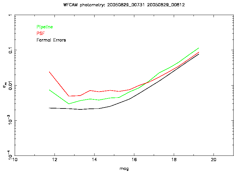
Figure 8: This plot shows the relative photometric errors as a function of
magnitude for the 2x2 UDS test.
Figure 9: This plot shows the relative photometric errors as a function of
magnitude for the 3x3 UDS test.
Tests have been carried out using data covering M17 in order to test the
performance in more crowded fields. 97 frames were measured with no failures
in the PSF measuring procedure. This shows that the methods used to
eliminate the effects of contamination work well.
Using data from the best seeing conditions (0.7") and comparing JHK
colour-colour diagrams it can be seen that the pipeline and PSF photometry
have similar accuracies. However, in worse seeing conditions (0.8-1.0"),
it is seen that the PSF photometry does not perform as well as that from the
standard pipeline. Close inspection of the images used indicate that the PSF
may be varying between each of the interleave stages and this could be the
cause of these problems. Alterations to the PSF measuring algorithm to take
this into account are in progress.
Further work is also required in accounting for the correlations with the
contaminants when carrying out the astrometric determination. The current
algorithm uses a "clean"-type method. A multiple component algorithm will
take correlations of the contaminants into account.
In carrying out these tests photometric non-linearities, possibly linked to
the weighting scheme used, showed up. Further investigations into these are
ongoing.
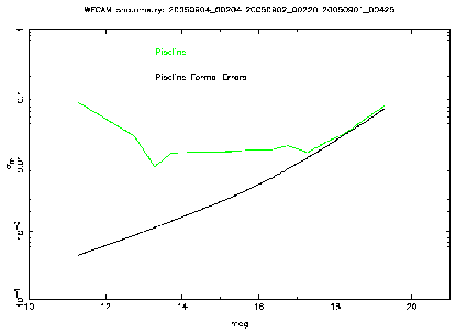
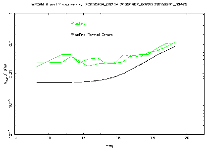
8 Error estimates on some standard pipeline values
Using the same procedure used to measure the astrometric and photometric
errors in Section 3, the quoted pipeline errors were compared.
Figure 10 shows typical results from these tests.
At the bright end, both astrometric and photometric errors level off to
constant values, probably caused by turbulence in the
atmosphere. The quoted errors do not reflect this. The faint end quoted
photometric errors match the measured errors very well, but for the
astrometry the quoted errors at the faint end tend to be underestimated.
Some comparisons have been carried out in crowded fields. In this case the
astrometric errors performed better at the faint end. However, one of the
frames exhibited a large magnitude term in y amounting to 0.05 pixel (20
mas) over the observed magnitude range. A visual check of the data did not
reveal any obvious problems with the images.
Figure 10: A comparison between measured and quoted astrometric and
photometric errors from the pipeline reductions.
The model used for the PSF comes from the adaptive kernel method used in
[Alard & Lupton 1998]. In this model a number of modified Gaussian profiles are
added together. The modification consists of multiplying them by polynomials
of varying degree. The advantage of this model is that the fitting process
is a linear least-squares problem.
K=
∑
n
∑
i
∑
j
ak e-(u2+v2)/2σn2uivj
Three Gaussian profiles were chosen for the PSF model.
The choice of σn to use is important to the success of the fit. It
was found that if the peak of the PSF was central, then the fit will be good
if the width of the PSF is between the width of the first and third Gaussian
profiles. If the PSF has a slight offset, then the width of the
central Gaussian profile should be close to the width of the PSF. Using the
half-width half-maximum (σp) value of the PSF to scale the
widths of the Gaussian
profiles the values used are σ1=0.3σp, σ2=0.9σp
and σ3=1.8σp.
For the first and second Gaussian profiles polynomial multipliers up to
fourth order are used. For the third up to only second order are used.
This implies fitting a model with 36 coefficients to the PSF.
File translated from
TEX
by
TTH,
version 3.30. On 17 Jan 2006, 10:48.