The purpose of this document is to investigate the photometry that can be
obtained from direct PSF fitting of simulated WFCAM data and generating
well-sampled PSFs or model-fitted equivalents.
The underlying
problem of this task is that the data is undersampled. The median seeing is
expected to be 1.5 pixels.
It is intended that the development of PSF fitting within the WFCAM project
be carried out in 3 phases:
List-driven - the X and Y positions are determined using
intensity-weighted centroids from the standard
CASU pipeline software with the photometry determined by PSF fitting using
these positions.
List-driven with positional updating - as in the previous case, but
the positions are iterated around the given position to determine the best
PSF fit, yielding both photometry and astrometry.
Full PSF fitting - the use of PSF fitting to
improve detection, astrometry and photometry
This document describes Phase 1 of the development.
A good paper to read on this topic is [Anderson & King 2000] and a number of ideas are
used from it, especially the use of the effective PSF.
The source data used in these tests were the same simulations as generated
in [Evans 2003].
However, only two sets of simulations were used in these tests:
Interleaved data, with all four elements of the interleaved
images generated with the same seeing (0.6").
Non-interleaved data with the same total integration time as above.
The simulations were carried out down to J=22.2, so that some of the effect of
undetected faint stars could also be accounted for (the detection limit is
about J=20 [Irwin 2003]).
Also, some simulations were carried out for low galactic latitudes, with
10 times the image density of the above simulations, to see if
crowding is likely to cause any problems.
The methodology used is fairly simple with the primary assumptions that:
All stellar positions down to a limiting magnitude are known.
The PSF for each star is known.
After a suitably binned PSF is generated for each detected star, a
least-squares solution is applied to determine the flux level for these
stars.
Using a list of detected stars (generated by another part of the pipeline),
each star is processed in turn. A cutout is made around the star from the
image data. Then, correctly sampled PSFs are generated for each star within
the cutout that might affect the flux levels. The least-squares solution is
generated from this subset of the data and using these PSFs.
The PSFs for the fitting were generated by bilinearly interpolating an
oversampled PSF which was calculated using the data from the whole image. It
was found very early on that using a simple scheme where the required PSFs
were calculated using the nearest neighbour values from an oversampled PSF
was not sufficient, even though the PSFs generated looked reasonable by eye.
This was necessary, not only for determining the PSFs of the primary star in
the solution, but also for the PSFs of the perturbing stars.
The weighting used was inverse variance and thus the formal errors for the
photometry come from the inverse matrix and χ2 values determined in
the least-squares solution. Tests were also carried out with uniform
weighting where the results were dependant on whether the data was
interleaved or not. Further tests on this aspect will be carried out when
real data is available from the telescope.
The flux levels of the perturbing stars in each cutout are not kept since
they may not be the most reliable measures - especially if they
intersect the edge of the cutout. Although this may not be a very efficient
method of implementing the solution it has advantages while developing the
software.
The effect of the stars fainter than the detection limit was to add to the
background level. The background level can be solved for as part of the
least-squares solution. However, in this investigation it was found that
having the background as part of the solution introduced systematic errors
at the faint end. A better result was found by taking the median pixel value
of the cutout ie. determining it globally.
It should be noted that photometry of the faintest images
from PSF fitting is fairly sensitive to the background determination.
Since WFCAM has not been commissioned yet, there is no test data available
to determine if there is an easy parametric model to use for the PSF. The
simulated data uses a Moffat profile to define the PSF, but this may not be
what is found in the real data. Thus, a non-parametric scheme was initially
devised to measure the PSFs from the image data. This is the same approach
as used in [Anderson & King 2000].
The model is simply a 2d pixel map of the PSF with an oversampling ratio of
5. In this scheme the information from the standard CASU pipeline is used to
determine which images to use and where to add the data. After the sky has
been removed from the data, the images selected must be:
within a specified magnitude range (currently between 1.5 and
8 magnitudes above the detection limit (S/N=5))
classified as a star
below an ellipticity limit - this is to reject certain types
of merged images
not close to the edge of the frame
have no very close neighbours
have no bad pixels within the contributing area
have a peak height that is not above saturation limit
The measured x and y information for each image is used to interleave
the image into the oversampled PSF image. The normalization of the PSF
is done using the standard pipeline aperture photometry estimate of the flux
for each of the contributing images that have gone into the PSF. The averaging
carried out for
each cell within the 5×5 grid is a median. This provides a robust
estimate which can deal with the occasional contaminating nearby image.
Another advantage of this approach is that when constructing the PSF in this
manner, the integration over a pixel has already been carried out. This
means that during the fitting stage, to generate the PSFs for each star, you
do not have to carry out any integration over a pixel, thus saving
considerably in CPU time. It should also be noted that because of this, the
sampled PSF will not be a match to the underlying PSF, but this is not
necessary for the fitting process.
Before the PSF estimation is carried out the the sky level is removed from
the frame and at the end a Hanning filter (also known as a 3×3
Bartlett filter)
[
1
2
1
2
4
2
1
2
1
]
is applied to the oversampled PSF. A smoothing kernel, as described in
[Anderson & King 2000], was also tried out but didn't give significantly different results.
The above estimation does not take into account the PSF possibly varying
across the field of view. However, a separate PSF will be generated for each
chip for each exposure.
The first tests were carried out using perfect, rather than measured,
PSFs. These were generated
using the same parameters as went into the simulations. The purpose of this
was to test the PSF fitting programme and thus separating the testing of the
two problems of measuring and fitting the PSFs.
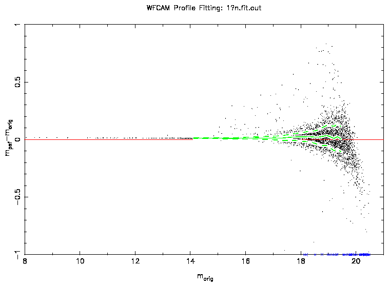
Figure 1: A plot of the difference between the original and measured
PSF magnitudes using a perfect PSF. The green solid and dashed lines show
the median and widths of the distribution. The extreme outliers are caused by
mismatches between the original and measured positions. The data shown here
is the non-interleaved data.
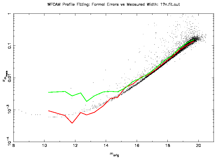
Figure 2: This plot shows the width of the distribution from
Figure 1 (red) along with the equivalent measure for aperture
photometry (green). Also plotted are the formal errors from the PSF fitting.
Figure 1 shows the difference between the original and
measured magnitudes using a perfect PSF, in this case a Moffat profile with
α = 0.75 and β = 2. A slight offset of 0.01m is seen which could
be due to detailed differences between the simulation and fitting
programmes in the way that they use the profiles. An offset should not cause
any problems in the end photometry since this should be taken care of by the
calibrations. These will be carried out using the aperture photometry and
all that will then be required is to determine the offset between the
aperture and PSF-fitted photometry.
Figure 2 shows the width of this distribution (a measure of
the accuracy) along with the equivalent error estimation for aperture
photometry (generated by the standard CASU pipeline). At the faint end the
accuracy of PSF fitting is slightly better than that of aperture photometry
which is due to the use of profile information.
At the bright end, the
accuracies should be comparable, however, in the example shown, the aperture
photometry does not perform as well due to the undersampled nature of the
data. The aperture calculated is affected by pixellation at the edge of the
aperture. Even though a soft-edged aperture is used,
it is affected by the undersampling.
For the interleaved data, the bright end
performance is comparable between aperture photometry and PSF fitting using
a perfect PSF.
Also shown are the formal errors resulting from the least-squares solution.
This shows that, given that the PSF is well known, the formal errors are a
reasonable estimate of the true errors in PSF fitting.
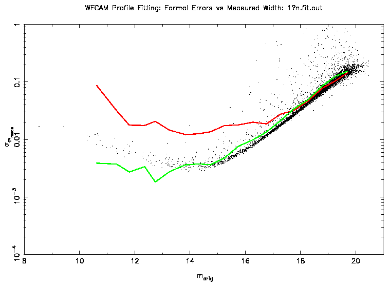
However, an accurate determination of the PSF is crucial. Using the
measuring scheme outlined above to determine the PSFs, a similar analysis
was carried out (see Figure 3). Fainter than 15-16m, the
results are broadly similar. Brighter than this and the magnitudes derived
from profile fitting have much worse errors than previously (more than a
factor of 10).
Figure 3: This plot shows the same analysis as Figure 2, but
using a measured PSF. The green line (aperture photometry) is the same as in
the previous plot.
Many investigations were carried out to identify the cause of the poor
performance of the PSF fitting. A possible cause could be the fitting
algorithm
itself, since it uses positions which which have associated errors.
However, this was quickly
eliminated since the use of the perfect PSFs gave good results, which leaves
us with the process of measuring the PSFs.
The measuring of the PSF uses derived information from the standard pipeline
which will have an associated error with it, specifically, the astrometry
and the star/galaxy classifier. The effect of errors on both of these
will be to broaden the measured PSF. However, tests using perfectly known
astrometry and classifiers yielded very similar results.
This leaves noise in the measured PSF as the possible source of the errors.
This can have two possible contributions: noise from the pixel counts and
"shot noise" from the limited numbers of clean stars to use within each
element of the interleaving grid. However, the contribution of the latter
will be small due to the robust nature of the averaging, so that even
slightly contaminated images can be used, thus increasing considerably the
number of stars available.
In order to reduce the noise level of the measured PSF, smoothing can be
carried out. However, this will usually broaden the PSF and reduce its
effectiveness as a representation of a point source. Another way is to fit a
function to the measured PSF. If the chosen function is a good
representation of the data then this effectively smooths the data without
broadening it. In these tests, we used a Moffat profile as a good general
function to do the fitting. Note that a Moffat profile will not provide a
perfect fit to the measured PSF due to the interleaving that has occurred to
the data. For Phase 1 and 2 a good approximation to the profile is all that
is needed.
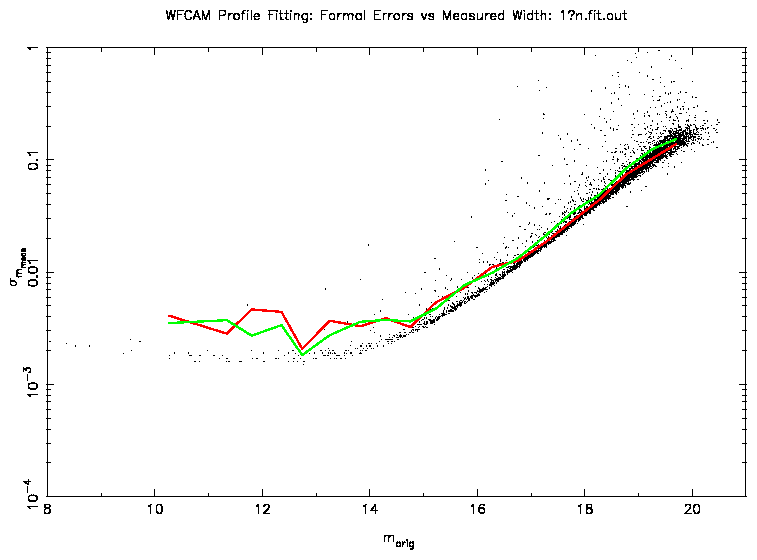
Figure 4 shows the results of using this parametric PSF in
the fitting programme. The errors at the bright end are much better than
before although not quite as good as when using the perfect PSFs
(Figure 1). The finding that a parametric PSF is the best
option is different to that found in [Anderson & King 2000] where they state that an
analytic PSF representation lacks the necessary flexibility. Their sampled
PSF turns out very smooth and yields good results. The difference is
probably due to the larger number of stellar images available for the
determination of the PSF. They have 3000 images in each of their 15 frames
and the PSF is assumed constant between them. However, since they have a
spatially varying PSF, this number should be divided by 9. By comparison,
the WFCAM images will have about 500 images per exposure.
Figure 4: This plot shows the same analysis as Figure 3, but
using a parametric PSF. The green line (aperture photometry) is the same as
in the previous plots.
The scheme outlined here is more robust than fitting a Moffat profile
directly to the data in order to determine a parameterized PSF. This is
because contaminating images are dealt with early on in the process before
the fit is carried out. However, is is possible that for determining a PSF
that is varying across the field a more direct PSF determination may be
necessary.
Tests were also carried out on the effectiveness of PSF fitting in crowded
regions. Using 2MASS source counts to estimate the number of objects at low
Galactic latitude, the number density of stars was increased by a factor of 10.
Using the PSF scheme outlined above, the performance of the PSF fitted
photometry matched that of aperture photometry. In comparison with the
non-crowded tests, the photometric accuracy was about 30% worse except for
the bright end where the accuracies were comparable.
In order to test the software further, INT Wide Field Camera data of the
Wolf-Lundmark-Melotte (WLM) galaxy in the Local Group was used. Three frames
in each of the passbands
Harris V and
Sloan i' were analysed. By using 3 frames it is possible to determine the
external photometric errors for each frame
by making the assumption that the width of the
residuals in any comparison is equal to the quadrature sum of the external
errors for each frame. With 3 frames it is possible to generate 3 sets of
residuals and thus determine what the external errors are by solving the
simultaneous equations.
This also assumes that the errors are not correlated ie. independent.
A weakness of this
method is that the measurement of the widths of the distributions is quite
noisy and the nature of the equations amplifies this.
Sometimes solutions are not possible due to this noise.
Often 2 frames taken in similar conditions is enough to determine the
external errors by assuming that they are the same for both frames.
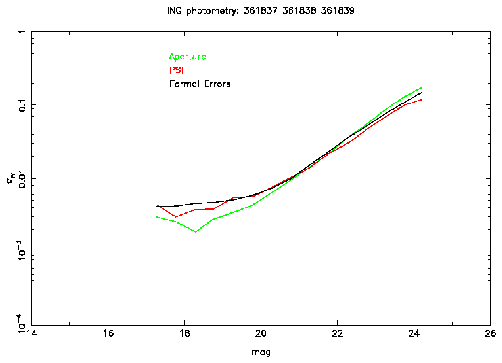
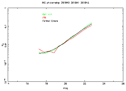
Figure 5 shows the measured errors for PSF and aperture photometry
along with the formal errors from the PSF fitting. This shows similar
results to that from the simulated data in that there is a comparable
performance between the PSF and aperture photometry at the bright end and
that at the faint end the PSF fitted photometry performs slightly better.
Also the formal errors are a good estimate of the true errors.
In these tests we used both circular and elliptical Moffat profiles with the
latter performing marginally better.
Figure 5: This plot shows the external errors for PSF (red) and aperture
(green) photometry as a function of magnitude
for data taken with the INT Wide Field Camera.
The V band is on the left and i' on the right. Also shown are the average
formal errors as a function of magnitude (black).
This work shows that the performance of PSF fitted photometry, using the
described scheme, is as good as that of aperture photometry at the bright
end and slightly better at the faint end.
Future work:
Effect of interleaving on profile fitting. Use of realistic seeing
conditions - perhaps measure the PSF separately for each contributing frame
and then interleave these to make the PSF used for the fitting of the
interleaved frame.
Effect of interpolation on profile fitting.
Further parameterization of the PSF determination.
Take into account the PSF varying across the field of view.
Investigate weighting options further when real data is available.
In the following sections, the definitions of the Moffat profiles used are
given along with the derivatives that are needed for the non-linear
least-squares solution.
In order to simplify the equations used, the circular Moffat profile is
defined by the formula
Ir=I0
⌈ ⌊
1+
⌈ ⌊
r
α
⌉ ⌋
2
⌉ ⌋
-β
where r is the radius, I0 the peak value, β the atmospheric
scattering coefficient and α is related to the half-width
half-maximum of the profile by the equation
α =
hwhm
√
2[ 1/(β)]-1
The required derivatives of the defining formula are
where Cartesian coordinates (x,y) are used rather than radial. How the
shape parameters (axx, axy and ayy) are related to the
ellipticity and position angle is given in the next subsection.
The required derivatives of this formula are
A.3 Initial values to enter elliptical Moffat profile fit
The non-linear least-squares solution can be speeded up by a factor of
~ 3 by starting off with good estimates of axx, axy and ayy.
Calculating the parameters
ellipticity (ell), position angle (θ) and number of pixels above
threshold, in a manner similar to that used by the standard pipeline
(see
http://www.ast.cam.ac.uk/~wfcam/docs/newparams3.ps)
you can obtain good initial values for the shape parameters
axx
=
Acos2θ+Bsin2θ
ayy
=
Asin2θ+Bcos2θ
axy
=
2(A-B)cosθsinθ
where A=1/a2 and B=1/b2 (a and b being the semi-major and
semi-minor axes respectively). These can be calculated from the relation
ell=1-b/a and setting the area of the ellipse (πab) to be equal to
the number of pixels above threshold.
File translated from
TEX
by
TTH,
version 3.30. On 26 Nov 2004, 13:32.