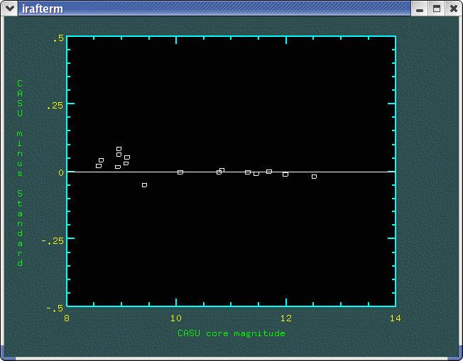
A comparison of core magnitudes
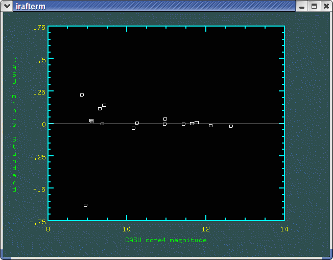
A comparison of core4 magnitudes
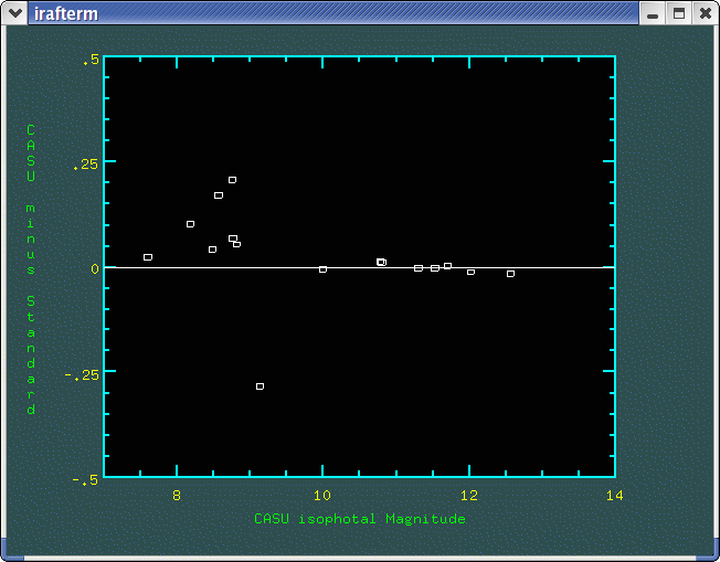
A comparison of isophotal magnitudes
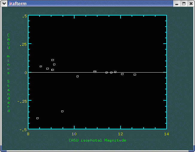
A comparison of total magnitudes
Apart from getting the right answer, the WFCAM pipeline must also run at the summit with the data reduction environment that currently exists at UKIRT (ORACDR). Non-WFCAM data can also be use to test whether the implementation of the WFCAM software has been done correctly within ORACDR.
In this paper I will present the results of some of the tests we have done on the WFCAM pipeline software. As more tests are finished then they will be added, hence the word 'draft' near the title above.
The CASU pipeline has already been installed and tested at JAC within ORACDR as part of the testing programme. The source has been made available to JAC from a CVS repository.
As part of the testing procedure on both the pipeline modules and our ability to implement a pipeline in ORACDR, we decided to run a small amount of data through both pipelines. The tests consisted of reducing some jitter observations from a single night (20020426) with both pipelines and comparing them for speed and consistency of results. Given that both pipelines reduce the data in a very similar way, then the results in terms of the sky background, image shape, photometry and positional accuracy should be roughly the same. The data were chosen so that they use a fairly simple recipe (JITTER_SELF_FLAT).
The tests were run on a Dell Inspiron 8100 laptop with 512 Mb of internal
memory and a 1.2 GHz Pentium III chip. In order to cut down on the
amount of time spent plotting, the reductions were done without the ORACDR
GUI and without any image display. For reference, the command used
was:
%oracdr -ut 20020426 -loop list -list 1:4,36:60 -log s -nodisplay
In what follows, I will refer to the standard Starlink based UFTI pipeline as the 'Standard' pipeline. The second CIRDR based pipeline will be the 'CASU' pipeline.
Briefly, the recipe in the Standard pipeline does the following:
Running these frames (essentially, two jitter sequences and a set of
array tests) through both pipelines yielded the following timing results:
| Pipeline | Run time(s) |
| Standard | 354 |
| CASU | 174 |
Using this simple recipe the CASU pipeline runs about a factor of 2 faster. Whether this is the case generally is beyond the scope of this little test. It is, however, quite probably that a large amount of the difference is in the resampling that takes place in the Standard pipeline during the stacking phase.
In order to compare the photometric and positional consistency of the two reduction methods a catalogue was generated for each of the stacked images using the catalogue generation program from CIRDR (imcore). The catalogues were generated in the following way:
| Parameter | Description |
| X coordinate | The X coordinate of the object (pixels) |
| Y coordinate | The Y coordinate of the object (pixels) |
| Isophotal flux | The flux with the detection |
| Total flux | The total flux of the object (Kron style) |
| Core flux | The flux through an aperture of radius Rcore |
| Core 4 flux | The flux through an aperture of radius 2*sqrt(2)*Rcore |
| Object Ellipticity | An estimate of the ellipticity for each object |
| Gaussian Width | The equivallent Gaussian width estimate for each object (pixels) |
Note that imcore generates object brightness in terms of data numbers
rather than magnitudes. Magnitudes are generated for these comparisons
by 2.5*log10(counts), so that brighter objects have a higher magnitude.
In the residuals below the sense is always
CASU minus Standard. In what follows, for the sake of brevity, we restrict
the analysis to objects on the first image stack that was reduced (group
number 36). The other groups give similar results.
| Parameter | Mean Residual | Standard Deviation |
| X coordinate | 1.000 | 0.227 |
| Y coordinate | 1.070 | 0.146 |
| Isophotal Magnitude | 0.044 | 0.066 |
| Total Magnitude | -0.032 | 0.134 |
| Core Magnitude | 0.014 | 0.033 |
| Core 4 Magnitude | 0.032 | 0.068 |
| Gaussian Width | 0.057 | 0.096 |
| Object Ellipticity | 0.001 | 0.013 |
There is a significant mean residual in the x,y coordinates. This is simply an artifact of the different the stacking algorithms used and how the origin is assigned. The standard deviations in the coordinates are also a remnant of this, in that the Standard pipeline rebins using some form of interpolation, whereas the current CASU pipeline uses the nearest neighbour.
All of the magnitude estimates reproduce to a good level of consistency. The standard deviation of the larger aperture magnitudes increases due to the larger contribution from the (noisy) background. The large mean residual and standard deviation in the total magnitude estimate is caused almost entirely by two deviant points (two fuzzy images). If these are removed then they drop to 0.016 and 0.037 respectively.
Finally, the two shape parameters we have included, the Gaussian width and the object ellipticity both agree very well. The CASU objects appear to be slightly larger than the standard pipeline objects, which is to be expected given the 'nearest neighbour' rebinning scheme used by the CASU pipeline. The mean gaussian width for this particular tile was 2.20 pixels, hence this residual corresponds to roughly 2.5%.
Below are comparison plots for the four magnitude estimates we've included.

A comparison of core magnitudes

A comparison of core4 magnitudes

A comparison of isophotal magnitudes

A comparison of total magnitudes
Last modified: Mon Feb 16 16:50:22 2004