COSCIRP and cosmic ray rejection
Cosmic ray rejection becomes important for the 15min-30min exposures
usually performed with CIRPASS. Cosmic ray rejection is being
performed using the CIRPASS IRAF task
coscirp. A typical long exposure with CIRPASS is made up
of multiple loops of multiple read (since there is no penalty for
reading the array many times in None Destructive Read (NDR) mode).
Parameters for coscirp can be found here.
Coscirp simply differences adjacent loops in the
docirpass processed _ima.fits files and
combines the sub frames using IRAF IMCOMBINE with
crreject removing cosmic ray candidates based on known
detector noise characteristics.
The output file from coscirp is still a
_ima.fits file but contains only one science extension
[sci,1] (with the associated error arrays) rather than
the full set of individual loop extensions.
Coscirp can be run automatically when
docirpass is run or can be run after
docirpass depending on how the observations have been
taken. Check the output from docirpass. An example
output is shown here. If
coscirp has not been run the references to Running
cosmic and the IMCOMBINE information will not be
shown. Also check for the existence of a rejected pixel list file
such as rej_crsn1987a_5173_ima.1.pl. These pixel list files
should be examined in IRAF (display
rej_crsn1987a_5173_ima.1.pl) to make sure that a sensible
rejection has been performed.
Pit-fall : If for some reason you
try to run coscirp on a file that has already been
COSCIRPed the software will corrupt the data file and you'll
have to start again, delete the file and rejection mask and rerun
docirpass and coscirp. Hopefully some extra
error checking will be added here in the future.

Identifying the calibration fibres
Now run the CIRPASS
IRAF task FIBCAL to trace the positions of the
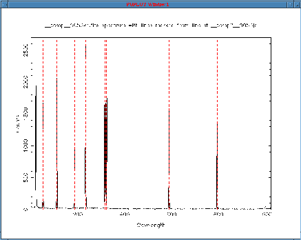
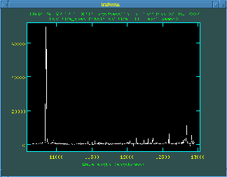
calibration fibres. The routine parameters can be found here. The routine displays a PGPLOT
window which shows the calibration fibres and their identifications if
the software has run correctly. Several of the calibration fibres are
poorly separated on the slit. These fibres may be missed or
incorrectly identified. However, the software knows which fibres
these are and deals with the situation correctly in most cases. The
Pit-fall to watch out for is the
correct first and second fibres are identified in the
fibcal task parameters.
The FIBCAL routine requires a text file with information
about the organisation and spacing of the fibres on the science array.
As measured for the 2002-3 observing runs the file can be found here. It is distributed with the
CIRPASS software tar file.
Pit-fall : There is a hidden
parameter that can be EPARed. It sets the width of the
fibre profiles when doing the optimal extraction. Check out the Pit-falls page for details.
|

|
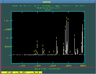
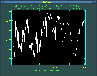
Pit-fall : The graphics output shown
to the left requires that the PGPLOT libraries are set up
correctly for the CIRPASS software. This can be complex
for some configurations. It is important to review this plot and
confirm that the correct calibration fibres have been identified. To
overcome potential problems with a users configuration an option exists
to write the information shown in the plot to a text file and suppress
the PGPLOT output. When running FIBCAL one
will be asked :
IRAF> View the 1st set of peaks found, text output otherwise? (yes)
By default answering yes displays the graphic using
PGPLOT. Answering no will suppress
PGPLOT and create/overwrite a text file fit.txt.
This file contains the data necessary to generate the
PGPLOT figure outside of CIRPASS IRAF. The
first 8 lines contain the centers of the calibration fibres in the 1D
cut across the array. The second part of the file contains the pixel
verses intensity spectrum along this cut. The user should confirm
that the fibre centers are correct by examining the data with an
external package (PGPLOT routine, IDL
etc...)

|
After accepting the fit (hit return in the IRAF window)
the traces are overlayed onto the calibration fibre image.
|
The headers of each image must now be updated to include a reference
to the new fibre id file (this should have been set at the
telescope).
Pit-fill : This step is
VERY important. If the wrong
fibpos file is used the reduction software will proceed
happily but the results will be rather meaningless.
hedit argon_5150*.fits EXTRFILE "fibpos_paschenJ.list" add- verify- show+ update+

hedit dome_51*fits EXTRFILE "fibpos_paschenJ.list" add- verify- show+ update+

hedit sn1987a*fits EXTRFILE "fibpos_paschenJ.list" add- verify- show+ update+

hedit hip022525*.fits EXTRFILE "fibpos_paschenJ.list" add- verify- show+ update+

hedit twilight_519*fits EXTRFILE "fibpos_paschenJ.list" add- verify- show+ update+

hedit twilight_520*fits EXTRFILE "fibpos_paschenJ.list" add- verify- show+ update+

Populating the Variance arrays
As of July 2003 the CIRPASS IRAF tasks use and propagate variance array information.
This information is used in optimal extraction and is also required for quantitative model fitting on the final
data sets. The task packages will work correctly without populating the error array (as they are, by default,
populated with 1.0) but inclusion of the error information is desirable. Significant gains in data reduction
and analysis can be made by propergating the error information.
At this time, limitations within the
IRAF IMCOMBINE task limit the accuracy with which this information can be propagated. It is
hoped that the CIRPASS reduction package will eventually have the IMCOMBINE dependance removed.
Flaws we have identified in the current strategy are highlighted below.
Variance information is generated based on the combined readnoise and Poisson noise of the recorded signal.
The unfortunately named IRAF CIRPASS task mkerr is used to populate the _ima.fits
file variance arrays.
mkerr mydata_ima.fits Readnoise Gain
Readnoise is given in electrons. The current measure value is 22.0. Some consideration must be give here to
the way CIRPASS data is taken. A single short CIRPASS observation is made up of a RESET frame
and a Science frame. The data stored in the _ima.fits file has been corrected for this RESET frame in a
manner similar to BIAS correction for CCD frames. The quoted readnoise is therefore the combined readnoise
of these two frames.
In order to reduce readnoise, CIRPASS science data (longer integrations on target)
are made up of a number of loops and reads. Loops are used to reject cosmic rays and should have been combined
with the COSCIRP task, leaving a data file which contains only one science extension
_ima.fits[Sci,1]. Each loop is made up of a number of detector reads (9 by default). Combining a number of
reads (using a simple average) reduces readnoise a factor SQRT(N). This step has been performed prior to
distribution of the data. For multiple read data the readnoise should be reduced by the SQRT(N) factor,
typical RDnoise=22.0/3.0=7.33.
The detector Gain is 7.0 e-/DN
NOTE : Due to the Hawaii array detector reset anomaly, all observations contain more than one detector read.
The first read of any integration is discarded. Typically CIRPASS data will be 2 Reads 1 Loop
(RDnoies=22.0 Gain=7) or 10 Reads 3 loops (RDnoise=7.33 Gain=7).
NOTE : The COSCIRP cosmic ray rejection task use IRAF IMCOMBINE CCDCLIP to reject
pixels from outside the noise model for the detetor. Where a pixel is rejected the subsequent data is scaled
for the missing pixel. There is currently no mechanisam for propergating this information and so the
Poisson noise added by MKERR will be an underestimate of the true noise in the scaled
pixel when a pixel as been rejected.
Image arithmatic
Images can be beam switched using the MEFARITH task as described below.
For _ima.fits files MEFARITH will correctly handle the variance array manipulations.
For _ms.fits files the new task MEFARITH2 handles the alternate file format.
In time, these two tasks will be merged into a single task which can identify the data type.
Application of flat fields
Generating useful variance information in flat field frames in difficult. However, the assumption that the
flat field frame(s) are not a major source in the error budget is fundamental for much of the data processing.
Therefore the current recommendation is that the variance arrays in flat field frames should be set to
0.0 NOT 1.0. Flat field frames should be created in the manner described below and MEF files created suing
the MAKEMEF tasks. The OVERWITE_EXT task should then be used to overwrite the
variance array with a 0.0 image. The MEFARITH and MEFARITH2 will then scale the
variance arrays when flat fields are applied to the data.
makemef template_ima.fits det-flat.fits det-flat_ima.fits

imdel temp.fits

imcalc det-flat_ima.fits[var,1] * 0.0 temp.fits

overwrite_ext det-flat_ima.fits temp.fits var 1

imdel temp.fits
NOTE : The fibre-to-fibre flat field is applied after extraction (ie to the _ms.fits files using
MEFARITH2. When extracting the fibre flat the variance array should be set with
MKERR using appropriate values for the readnoise based on the number of image combined.
The extracted _ms.fits file should then have it's variance array set to 0.0
Transformation information
For some, but not all, projects it is desirable to transform the extracted spectra onto a single
wavelength scale. While this step introduces correlated noise in the data, in most cases this correlation
will most likely not be a significant increase in the noise, and the transformation allows a better
background subtraction.
The variance array information must also be transformed in order to be useful.
While simply applying the same transformation as we used for the science data is
clearly not ideal (since it relies on every pixel in the transformation having an independent error)
to first order it does yield excellent results.
The process should be undertaken as follows
transform image_ms.fits[sci,1] sci.fits template.fits

transform image_ms.fits[var,1] var.fits template.fits

makemef3 image_ms.fits sci.fits sci_ms.fits

overwrite_ext sci_ms.fits var.fits var 1

Fixing bad pixels
A bad pixel mask is required to fix bad pixels to prevent them
interfering with the extraction routine. This is probably best
produced from a combination of detector flats and dark frames.
Current thinking is to take a long dark frame. Process for cosmic ray
rejection with COSCIRP as usual. Using IMSTAT,
GSTAT and/or IMPLOT an estimate of the background
level for good pixels can be made. IMREPLACE can then be
used to make a bad pixel mask image and pixel list.
imreplace.images = "badpix"

imreplace.value = 0.

imreplace.imaginary = 0.

imreplace.lower = INDEF

imreplace.upper = 200

imreplace.radius = 0.


imrep

imreplace.images = "badpix"

imreplace.value = 1

imreplace.imaginary = 0.

imreplace.lower = 200

imreplace.upper = INDEF

imreplace.radius = 0.


imcopy badpix.fits badpix.pl
|
|
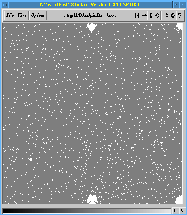
| A Problem with this step is that the
regions affected by amplifier glow may be rejected as bad pixels when,
in fact, beam switching does an acceptable job of correcting much of
these regions.
If bad pixel masking is done without accounting for this then some
information will be lost form some spectra at the ends of the IFU.
The workaround is to remove these regions form the bad-pixel mask,
assuming that the good data retained is preferable to the removal of
the few bad pixels in these regions. On beem-switching much of the
amplifier glow is cancelled out and only a small number of bad pixels
will remain.
|

|
To mask out the regions use IMCALC, with
suitable radius and offset parameters for the amplifier glow regions,
as follows :
|
imcalc badpix.fits badpix2.fits "if sqrt( (x-512)**2 + (y-0)**2) .lt. 50 then 0.0 else im1"

imcalc badpix2.fits badpix2.fits "if sqrt( (x-512)**2 + (y-1024)**2) .lt. 50 then 0.0 else im1"

imcalc badpix2.fits badpix2.fits "if sqrt( (x-1024)**2 + (y-0)**2) .lt. 50 then 0.0 else im1"

imcalc badpix2.fits badpix2.fits "if sqrt( (x-1024)**2 + (y-1024)**2)
.lt. 50 then 0.0 else im1"
The bad pixel mask is then used with the IRAF fixpix task.
|
Pit-fall : Frames must have bad
pixels fixed in such an order that all frames from which spectra are
to be directly extracted do not have additional defects added by
performing steps in the wrong order. Some checking still needs to be
done here to make sure we know the correct order.
fixpix argon_5150*_ima.fits[sci,1] bad_pix1.fits linterp=1  cinterp=2 verbose=yes

fixpix dome_51*_ima.fits[sci,1] bad_pix1.fits linterp=1  cinterp=2 verbose=yes

fixpix sn1987a*_ima.fits[sci,1] bad_pix1.fits linterp=1  cinterp=2 verbose=yes

fixpix hip022525*_ima.fits[sci,1] bad_pix1.fits linterp=1  cinterp=2 verbose=yes

fixpix twilight_519*_ima.fits[sci,1] bad_pix1.fits linterp=1  cinterp=2 verbose=yes

fixpix twilight_520*_ima.fits[sci,1] bad_pix1.fits linterp=1  cinterp=2 verbose=yes
Currently the interpolation over bad pixels is done along the x
direction which is roughly the spectral direction since adjacent data
pixels in the y direction are not physically associated with a point
on the sky.

Detector flat fields
A detector flat field is required to account for pixel-to-pixel
variations in sensitivity. Currently this is performed using a
combination of back illumination within the CIRPASS cold room and dome
flats taken with the spectrograph out of focus. Both scenarios yield
reasonable smooth background illumination from which to compile a
detector sensitivity image. Back illumination frames seem to work
best as there is then no imprint of the fibres on the detector.
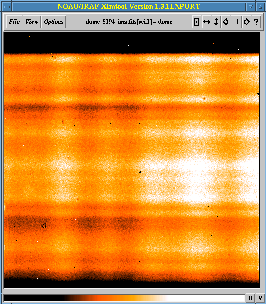
Defocused dome flats
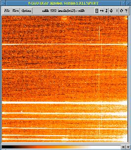
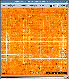
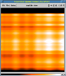
The raw frame shown to the left is block averaged in both dimensions
to produce a smoothed background frame. Since there is only one loop
to each frame multiple frames can be combined to remove any transient
effects. IMCOMBINE is used with the
crreject option. The parameter file can be found here Note that scale has been set
to none and zero is set to mode to account
for differences in the illumination level, these parameters need to be
adjusted as appropriate every time IMCOMBINE is used.
One should check that all the exposures used are at the correct level
(light level tests often mean the first few exposures are too high or
too low). |  |
imcomb @list_outoffocus outoffocus_sky.fits scale=none zero=mode

makemef dome_5191_ima.fits outoffocus_sky.fits outoffocus_ima.fits
Since IMCOMBINE
is a standard IRAF task, the images require the extension
to be given and so IRAF @listlist_outoffocus looks like:
|
dome_5191_ima.fits[sci,1]
dome_5192_ima.fits[sci,1]
dome_5193_ima.fits[sci,1]
dome_5194_ima.fits[sci,1]
|
Smoothing is accomplished with blkavg and blkrep.
|
|
imdel temp1.fits,temp2.fits,temp3.fits,temp4.fits,temp5.fits

blkavg outoffocus_ima.fits[sci,1] temp1.fits option="average" b1=1 b2=1024

blkrep temp1.fits temp2.fits b1=1 b2=1024

blkavg outoffocus_ima.fits[sci,1] temp3.fits option="average" b1=1024 b2=1

blkrep temp3.fits temp4.fits  b1=1024 b2=1

imarith temp2.fits * temp4.fits temp5.fits
|
The stacked flat frame is then divided by the smoothed frame.
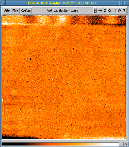
imarith outoffocus_ima.fits[sci,1] / temp5.fits bad_pix_flat.fits
|
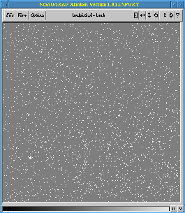
The result of this procedure is a mostly flat image with the bad pixel
highlighted. This process is performed with uniformly illuminated
back illumination frames.
|
 |

Wavelength calibration
|
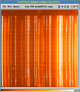
Next, extract the argon lamp exposure. The raw file shows the spectra
curvature across the chip. Calibration is best done using airglow
lines within sky frames of the science data. However, argon lamp
frames are required during the instrument set up and can be easier to
identify to provide a first pass at the wavelength solution.
We use optimal extraction rather than much quicker
summed extraction, as was most likely done at the telescope.
The routine parameters can be found here.
|
=
|
dot argon_5150_ima.fits extract=opt interac=no
|
Turning the interactive option off prevents dotarget from
running IDISPLAY and showing IFU image
reconstructed from the _cal.ms.fits file. If this is
left active, then at the end of the reduction, you must quit
IDISPLAY to return to the cl prompt.
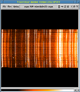
The resulting extracted spectra multi-spec image is shown to the right.
|
|
Next the spectra need to be wavelength calibrated with
identify. There is a glitch in IRAF here in
that while all the different spectral reduction packages
(ONEDSPEC, TWODSPEC ...) use the same
identify software, they all seem to use different
uparm parameter files and so if you change the line
list in identify you must ensure that the current version of
the identify parameters you are using have the correct line list.
Run identify with the parameters something like those given here.
imcopy argon_5150_cal.ms.fits[sci,1] argon.fits

identify argon.fits
Identify the spectra in the usual way.
Currently we have not compiled a set of CIRPASS reference spectra.
Try using the Gemini - UKIRT ones for now, http://www.gemini.edu/sciops/instruments/gcal/gcalArgonLamp.html
A Pit-fall here is that the lines
are labelled in microns with some of the lines having 6 digits and
some with 5. Since you want the line list in Angstroms you only want
to type the first 5 digits of the line ID. The decimal point
precision is not generally needed since identify will
find this, a good check that it is working properly. |  |
Pit-fall : There are some funny
features with identify that are not yet fully understood. Once the
spectra are identified an IRAF database entry is writing
for the file but WCS information is also written to the file header.
This WCS information seems to confuse later tasks such as
REIDENTIFY and transform. Simply removing
all of the WCS information that identify adds to the file seems to fix
the problem. More information on this will be added as more is
uncovered.
Next, run REIDENTIFY to fit the wavelength solution across the full
image. Parameters are here.
The next step is to run FITCOORDS to fit the 2D solution
across the spectral image. param. One
problem that I found is that the image to be fitted must be given
without the .fits or the task will fail to find the right
data base file. Details of how to run FITCOORDS can be
found in the IRAF tutorial 'A User's Guide to
Reducing Slit Spectra with IRAF' in the appendix on
reducing LONGSLIT data.
A reasonable fit seems to come with xorder=3 yorder=6 but more work on this is needed.
Using this solution one can then use transform to rectify
the spectrum. I'm not totally sure I've got the correct settings for
transform yet. param.
|
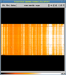
In the rectified image the argon lines have been straightened out.
There are some odd features which do not extend across the full width
of the spectrograph which are actually made worse by the
transformation. Currently the identity of these lines is not known
but they are most likely second order lines from strong optical argon
emission features.
|
 |

Twighlit flats
Twighlit flats provide an excellent
uniform illumination. First combine all the flat fields to make a
crrejected flat field frame. Do check that all the
frames are well exposed first though. Light level at the telescope
checks can lead to some poorly exposed frames. |
gstat twili*fits[sci,1]
| IMAGE | MEAN | MIDPT |
|---|
| twilight_5115_ima.fits[sci,1] | 1100.81 | 1087.98
| | twilight_5116_ima.fits[sci,1] | 837.155 | 822.205
| | twilight_5117_ima.fits[sci,1] |
558.731 |
545.138 |
| twilight_5195_ima.fits[sci,1] |
150.928 |
156.006 |
| twilight_5196_ima.fits[sci,1] |
227.415 |
234.909 |
| twilight_5197_ima.fits[sci,1] |
342.022 |
354.078 |
| twilight_5198_ima.fits[sci,1] |
497.272 |
517.931 |
| twilight_5199_ima.fits[sci,1] | 701.927 | 732.202 |
| twilight_5200_ima.fits[sci,1] | 918.023 | 959.095 |
| twilight_5201_ima.fits[sci,1] | 1207.33 | 1262.99 |
| twilight_5202_ima.fits[sci,1] | 1546.28 | 1623.12 |
| twilight_5203_ima.fits[sci,1] | 1833.50 | 1931.99 |
| twilight_5204_ima.fits[sci,1] | 2106.74 | 2225.13 |
| twilight_5205_ima.fits[sci,1] | 2314.64 | 2447.13 |
|
Combine the well exposed flats with imcombine.
|
imcomb @list_twilight twilight.fits scale=none zero=mode

makemef twilight_5115_ima.fits twilight.fits twilight_ima.fits
|
|
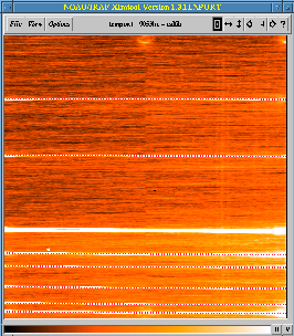
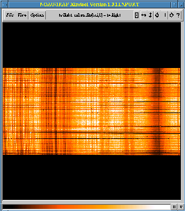
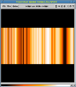
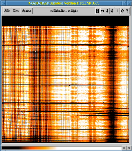
The combined image shows a heavily structured flat field made
containing the solar spectrum.
Now extract the target and the flat field spectra using optimal
extraction. This bit will take some time. Check at this point for
error messages. A common error is that the wrong or a missing fibre
position file, something like the fibpos_paschen.list used here
and created form the calfib_ima.fits image earlier, is
not correctly specified. Not specifying a file will result in no
extraction being done. Specifying the wrong file will happily extract
rubbish from the data and produce an _cal.ms.fits file
with some very odd spectra in it.
|
|
The flat field frame is not applied until after the spectral
extraction as this would corrupt the fibre profiles seen by the
detector which are required for the optimal extraction (Johnson
R. 200?).

Beam switching
A first order sky subtraction is achieved by subtracting offset sky
frames from the data. This step also suppresses the effects of amplifier glow and hot pixels.
mefarith sn1987a_5173_ima.fits - sn1987a_5175_ima.fits sn1987a_1_ima.fits

mefarith sn1987a_5174_ima.fits - sn1987a_5175_ima.fits sn1987a_2_ima.fits

mefarith sn1987a_5176_ima.fits - sn1987a_5177_ima.fits sn1987a_3_ima.fits

mefarith sn1987a_5178_ima.fits - sn1987a_5177_ima.fits sn1987a_4_ima.fits


Extracting the science spectra
Optimal extraction is used as before. Turning off interactive mode
suppresses the display of the reconstructed IFU image for batch
processing.
dot twilight_ima.fits extract=opt interac=no

dot sn1987a_1_ima.fits extract=opt interac=no

dot sn1987a_2_ima.fits extract=opt interac=no

dot sn1987a_3_ima.fits extract=opt interac=no

dot sn1987a_4_ima.fits extract=opt interac=no
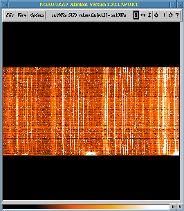
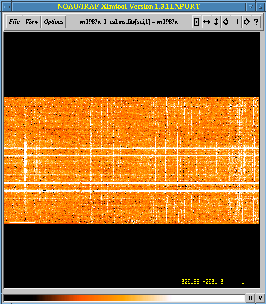
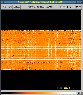
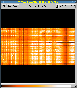
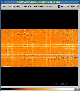
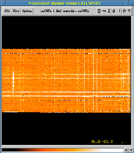
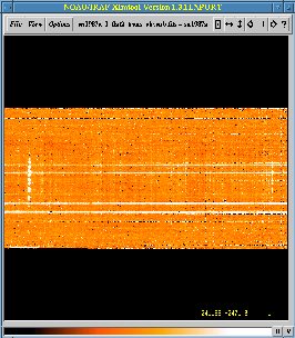
| Extracted spectra multi-spec files |
| Twilight flat |
Science frame without beam switching |
Science frame with beam switching |
 |
 |
 |
After extraction but before rectification with transform
the spectra are first pass flat fielded with the extracted flat field spectra.
imarith sn1987a_1_cal.ms.fits[sci,1] / twilight_cal.ms.fits[sci,1] sn1987a_1_flat1.fits

imarith sn1987a_2_cal.ms.fits[sci,1] / twilight_cal.ms.fits[sci,1] sn1987a_2_flat1.fits

imarith sn1987a_3_cal.ms.fits[sci,1] / twilight_cal.ms.fits[sci,1] sn1987a_3_flat1.fits

imarith sn1987a_4_cal.ms.fits[sci,1] / twilight_cal.ms.fits[sci,1] sn1987a_4_flat1.fits
|
Flat fielding in the somewhat unconventional maner is required for the
optimal extraction algorithm.
|

|
Transform the image in the same manner as the argon was. The twilight
flat field is also transformed.
transform sn1987a_1_flat1.fits sn1987a_1_flat1_trans.fits argon

transform sn1987a_2_flat1.fits sn1987a_2_flat1_trans.fits argon

transform sn1987a_3_flat1.fits sn1987a_3_flat1_trans.fits argon

transform sn1987a_4_flat1.fits sn1987a_4_flat1_trans.fits argon


transform twilight_cal.ms.fits[sci,1] twilight_trans.fits argon


|
Now a block averaged solar spectrum can be constructed from the
rectified flat field image to remove the solar spectrum component from
the flat fielded data. In principle the signature of the solar
spectrum (or the dome illumination) could be removed at the flux
calibration stage. I've found it easier to apply this first order
correction to remove most of the solar spectrum with the block
averaged spectrum here in most cases but more work on this is needed
to ensure data quality.
|
blkavg twilight_trans.fits twilight_spec.fits option="average" b1=1 b2=1024

blkrep twilight_spec.fits twilight_spec_2d.fits b1=1 b2=508
|
|
The flat fielded and rectified frames are then multiplied by this mean
solar spectrum to remove the solar spectrum from the data.
|

|
imarith sn1987a_1_flat1_trans.fits * twilight_spec_2d.fits sn1987a_1_flat2_trans.fits

imarith sn1987a_2_flat1_trans.fits * twilight_spec_2d.fits sn1987a_2_flat2_trans.fits

imarith sn1987a_3_flat1_trans.fits * twilight_spec_2d.fits sn1987a_3_flat2_trans.fits

imarith sn1987a_4_flat1_trans.fits * twilight_spec_2d.fits sn1987a_4_flat2_trans.fits

Residual background subtraction
Residual background subtraction can be accomplished using the IRAF
background task to subtract a polynomial fitted along each
column. Task parameters here. This step
works well with certain types of data but poorly with others. A guide
to when and how to do this is still needed.
|

|
background sn1987a_1_flat2_trans.fits sn1987a_1_flat2_trans_skysub.fits
background sn1987a_2_flat2_trans.fits sn1987a_2_flat2_trans_skysub.fits
background sn1987a_3_flat2_trans.fits sn1987a_3_flat2_trans_skysub.fits
background sn1987a_4_flat2_trans.fits sn1987a_4_flat2_trans_skysub.fits
Pit-fill : Note that to make the new
MEF file makemef2 must
be used since we want to make a _cal.ms.fits file NOT a
_ima.fits file.
makemef2 sn1987a_1_cal.ms.fits sn1987a_1_flat2_trans_skysub.fits sn1987a_1_flat2_trans_skysub_cal.ms.fits

makemef2 sn1987a_2_cal.ms.fits sn1987a_2_flat2_trans_skysub.fits sn1987a_2_flat2_trans_skysub_cal.ms.fits

makemef2 sn1987a_3_cal.ms.fits sn1987a_3_flat2_trans_skysub.fits sn1987a_3_flat2_trans_skysub_cal.ms.fits

makemef2 sn1987a_4_cal.ms.fits sn1987a_4_flat2_trans_skysub.fits sn1987a_4_flat2_trans_skysub_cal.ms.fits

Flux calibration with a standard star
The above steps are repeated on the standard star observations.
hedit hip022525*.fits EXTRFILE "fibpos_paschenJ.list" add- verify- show+ update+


fixpix hip022525*_ima.fits[sci,1] bad_pix1.fits linterp=1  cinterp=2 verbose=yes


dot hip022525_5179_ima.fits extract=opt interac=no


imarith hip022525_5179_cal.ms.fits[sci,1] / twilight_cal.ms.fits[sci,1] hip022525_flat1.fits


transform hip022525_flat1.fits hip022525_flat1_trans.fits argon


imarith hip022525_flat1_trans.fits * twilight_spec_2d.fits hip022525_flat2_trans.fits


background hip022525_flat2_trans.fits hip022525_flat2_trans_skysub.fits


makemef2 hip022525_5179_cal.ms.fits hip022525_flat2_trans.fits hip022525_flat2_trans_cal.ms.fits
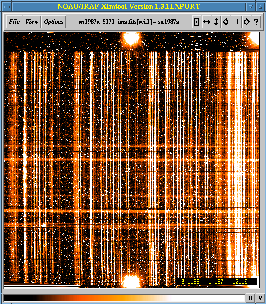
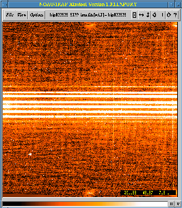
Raw _ima.fits file |
Optimally extracted multi-spec file _cal.ms.fits |
First flat fielding |
 |
 |
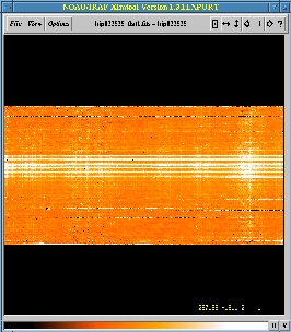 |
| After wavelength transformation |
Second flat fielding |
Background subtraction |
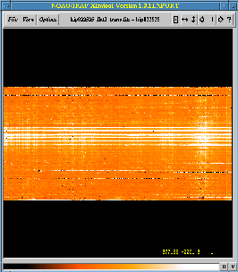 |
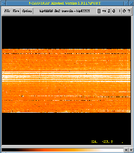 |
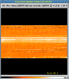 |
| Reconstructed short H band IFU image |
Combined spectrum |
|
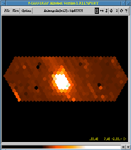 |
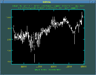 |
Once processed the standard star spectrum is produced by combining a
number of well exposed spectra from the IFU. A loss of total flux
results from including too few spectra. This must be balanced against
an increased noise which would result from adding too many spectra from
the wings of the seeing disk.
Several features are visible in the extracted spectrum which obscure
the underlying near black body spectrum expected for the standard
star. Features to be accounted for include the detector system and
filter response functions and Telluric absorption features. Stellar
absorption and emission features may also be present which need to be
removed from the response function. Producing a sensitivity function
from the extracted spectra can be done in a number of ways. An
IDL routine to allow interactive fitting of the
sensitivity function is under construction at Cambridge.

Mosaicing IFU data
Mosaicing is carried out using the CIRPASS IRAF mosaic
task. Inputs are list files for the images to be mosaiced and the
lens offsets of each images from a base position. A proper
description of how these offset are derived is still required.
Pit-fall : There appears to be a
slight problem with end of line characters in the input files where in
some case the wrong number of input images and offsets are read in.
Check the preamble that the mosaic task outputs to make sure it is
doing what you think it should be doing.
Pit-fall : If an already existing
image is given as the output image the software, which takes quite a
while to run, will not clobber the cutout and will simply crash out.
Check that the output image does not already exist.
mosaic images_to_mosaic lens_offsets_list output_image

mosaic sn1987a_mosaic.list sn1987a_offsets.list sn1987a_mosaic.fits
Pit-fall : IDISPLAY the
CIRPASS IFU reconstruction program has a slight bug in it which
results in small dark spots appearing in the display for mosaiced IFU
images due to the way the intermediate IFU image is generated. The
true image data is not affected and these spots are purely an artefact
of the display routine at this time.
Offset determination
Offsets are best determined from the image FITS headers.
hsel My-data*cal.ms.fits $I,INST_PA,LENS_SCL,OFF_RA,OFF_DEC yes


My-data*1*fits    90.00   0.25    -7.687  -8.660

..

..

My-data*N*fits    90.00   0.25    -7.687   0.000
The CIRPASS IRAF task LENSOFFSET can then be
used to determine the lens offsets between the data (taking care to
set the PA and LENS SCALE appropriately in the task.
Pit-fall : The Gemini Visitor
Instrument Interface (VII) return OFF_RA as a target coordiante offset
in decmial degrees. A correction for cos(DEC) is therfore required to
genearte the correct offset information.
Example :
TARG_RA = '161.27437500' / Target right ascension

TARG_DEC= '-59.66843333' / Target declination


hsel My-data*cal.ms.fits $I,INST_PA,LENS_SCL,OFF_RA,OFF_DEC yes

My-data*1*fits    90.00   0.25    -7.687  -8.660


IFU offset is = -7.687 * cos(-59.668) = -3.882

IRAF> lensoffset 3.882 -8.660 lens_sc=0.25 pos_ang=90 theta_o=0 PA_dire=1

Offset in lens units along the long axis, x = -31

Offset in lens units along the short axis, y = -40
|
The final extracted spectrum show several strong emission lines from
the region of the SN.
|

|

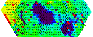
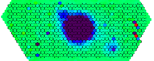
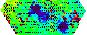
Reconstructed IFU images
Reconstructed IFU images show a variety of features. At the current
time the display software is a little limited.
More details about this object can be found at http://www.ast.cam.ac.uk/~rgs/cirpass_pub/index.php
| Full wavelength range image showing central SN and field
stars. |
Emission line image of SN1987a |
 |
 |
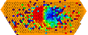
| Animation (click to run, then hit reload) showing the 2D image
in wavelength slices across the major emission line. |
A velocity map created based on the strong emission line form the animation |
 |
 |
Rob Sharp
<rgs@ast.cam.ac.uk>
Last modified: Mon Sep 9 17:30:45 2002


