Demo: Tidal Disruption Event

One of the recent applications of Python is modelling outflows in Tidal Disruption Events (TDEs). We have explored how line formation in an accretion disc wind could explain the BAL vs. BEL dichotomy observed in the UV spectra of TDEs. We have also explored how reprocessing in an accretion disc wring could give rise to the, at one point, unexpected optically bright TDEs.

We now describe a model used to simulate both the UV and optical features of TDEs.

Model Setup

Key Model Parameters

We model a disc wind outflow using the kinematic Shlosman & Vitello (1993) (SV93) biconical disc wind model. This model has seen extensive use throughout the history of Python to model across all length scales of accretion, from CVs to QSO winds. Further information about the SV93 model can be found in the documentation here.

The key parameters controlling the geometry and central object in this model are as follows.

Schwarzschild black hole parameters:

\[\begin{split}\text{R}_{\text{disc, in}} &=~10^{13} ~ \text{cm} \\ &=~22.8 ~ \text{R}_{\text{g}} \\ \text{R}_{\text{disc, out}} &=~10^{15} ~ \text{cm} \\ &=~2258 ~ \text{R}_{\text{g}} \\ \text{M}_{\text{BH}} &=~3 \times 10 \text{M}_{\odot} \\ \dot{\text{M}}_{\text{disc}} &=~9.99 \times 10^{-3}~\text{M}_{\odot}~\text{yr}^{-1} \\ &=~0.15~\dot{\text{M}}_{\text{Edd}}\end{split}\]

Wind geometry parameters:

\[\begin{split}r_{\text{min}} &=~10^{13} ~ \text{cm} \\ &=~22.8 ~ \text{R}_{\text{g}} \\ r_{\text{max}} &=~10^{15}~ \text{cm} \\ &=~2258 ~ \text{R}_{\text{g}} \\ \alpha &=~1.5 \\ R_{v} &=~5 \times 10^{16} ~ \\ &=~1.13 \times 10^{5}~\text{R}_{\text{g}} \\ \theta_{\text{min}} &=~20^{\circ} \\ \theta_{\text{max}} &=~65^{\circ} \\ \text{R}_{\text{max}} &=~5 \times 10^{17}~\text{cm} \\ &=~1.13 \times 10^{6}~\text{R}_{\text{g}} \\ \gamma &=~1 \\ \lambda &=~0 \\ f_{v} &=~0.1 \\\end{split}\]

For parameters controlling the radiative transfer and flow of Python, the parameter file for this model can be found here.

Radiation Sources

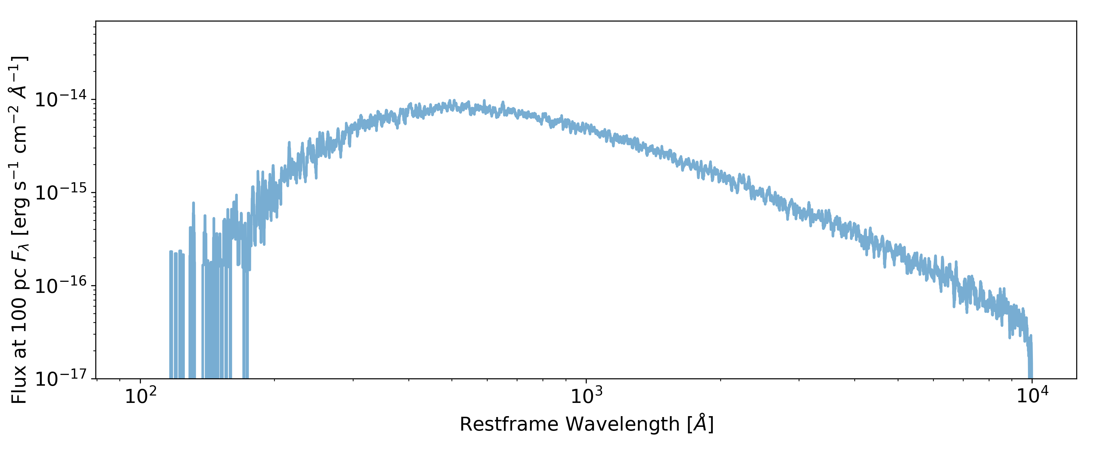
There are two radiation sources in this model; the accretion disc and the wind itself. Although, the wind does not act as a net source of photons, but rather as a reprocessing medium. We assume that the wind is in radiative equilibrium meaning any energy absorbed is reprocessed and re-radiated, i.e. via radiative recombination. We treat the accretion disc as an ensemble of black bodies, using a standard \(\alpha\)-disc effective temperature profile (Shakura & Sunyaev, 1973). The emergent SED is hence specified entirely by the mass accretion rate of the accretion disc and the mass of the black hole.

The figure below shows the angle integrated SED for this model.

The angle integrated accretion disc SED for the TDE model.

Runtime

As the TDE outflow is optically thick, the model requires a fair amount of computing power to be completed within a reasonable time frame. We ran this model using two Intel Xeon Platinum 8160 processors with 24 processor cores each for a total of 48 cores. Each processor core runs at a clock frequency of 2.1 GHz, with a maximum boost clock of 3.7 GHz. The model uses roughly 70 GB of the available DDR4 2666 MHz memory available in this system.

With this configuration using \(10^{8}\) photons and Python’s “-p 2” option for logarithmic photon number stepping, the model takes roughly 10 ionization cycles to converge in roughly 7.5 hours, or 360 total CPU hours. The spectral cycles take a significantly longer time to complete. For six inclination angles and \(10^{8}\) photons, a single spectral cycle takes in excess of three hours. However, with \(10^{6}\) photons a spectral cycles takes roughly 100 seconds. We find that 5 - 10 spectral cycles with \(10^{6}\) photons result in reasonable sacrifice between noise in the final spectrum and the run time of the spectral cycles.

Outputs

Synthetic Spectra

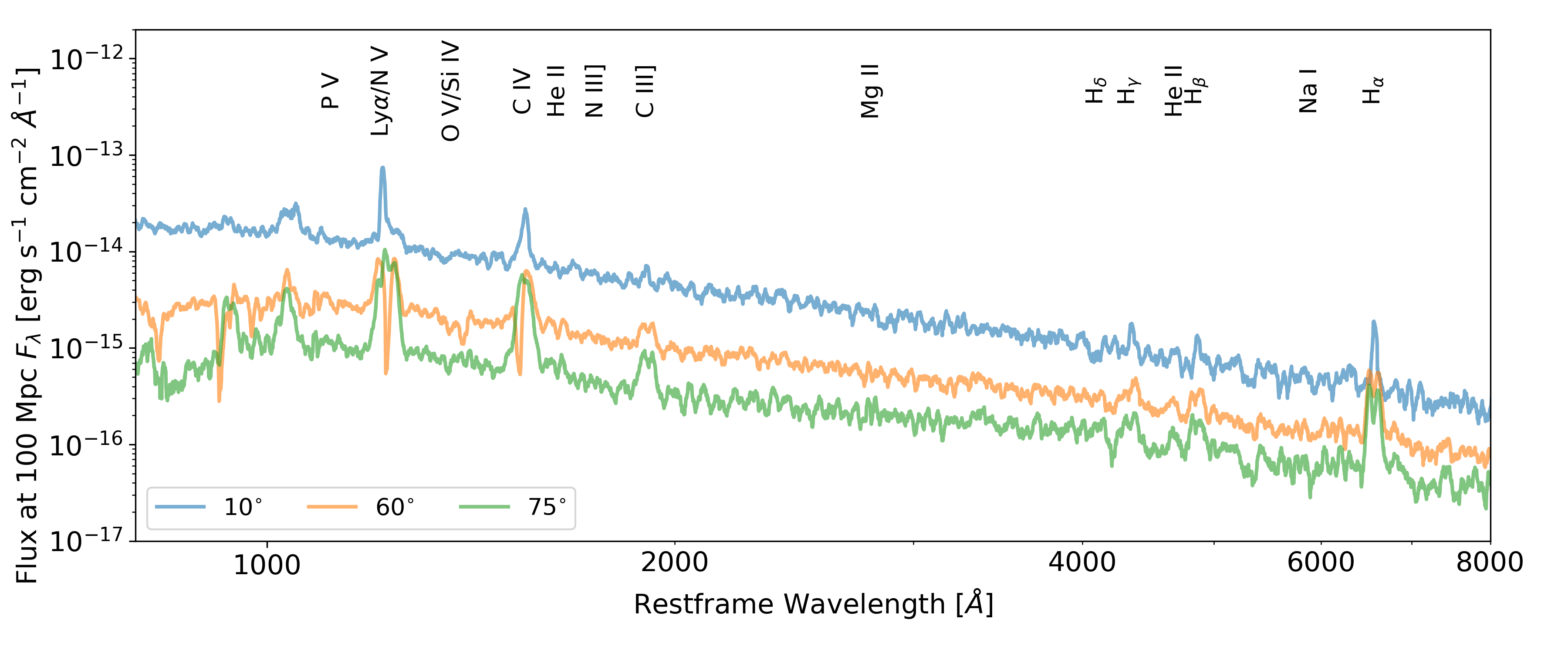
Below is a figure of three inclination angles of the emitted spectrum for this model.

Synthetic spectra of the TDE model for three inclination angles, as labelled in the lower left. The 60 \(^{\circ}\) sight line is looking down, into, the wind, whereas both noth the 10 \(^{\circ}\) and 75 \(^{\circ}\) sight lines are not looking above and below the wind respectively. Important line transitions have been labelled at the top of the plot.

The model produces the strong resonance lines of N V, Si IV and C IV often seen in UV spectra of TDEs and other objects with mildly ionized winds. We also reproduce the BAL vs. BEL behaviour seen, as described in, i.e. Parkinson et al. (2020),. For inclinations which look into the wind, BALs are preferentially produced and for inclinations looking above or below the wind, BELs are instead seen.

In the optical portion of the spectrum, the model produces broad recombination emission features for the Balmer series of lines as well as for He II. These features have extended red wings, clearest at low inclination angles. At intermediate and high inclinations, the emission features are double peaked due to the high rotational velocity of the wind near the base of the wind, where these features are forming.

Physical Properties

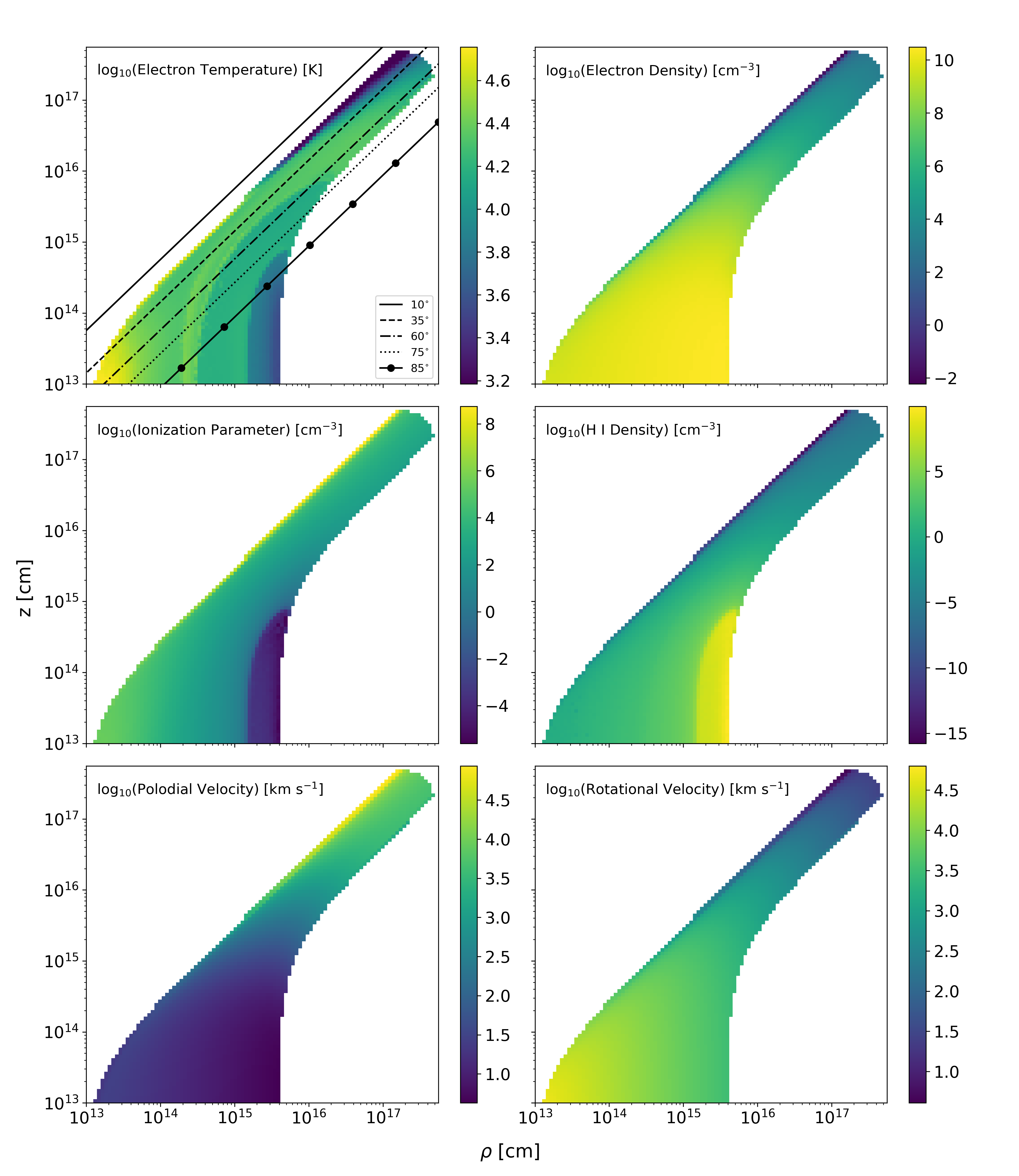
In the figure below, the physical properties of the outflow are shown.

Contour plots of various physical parameters for the wind model, plotted on a log-log spatial scale. The top left panel shows which parts of the wind four inclination inclinations intersect.

At the base of the wind, the velocity is dominated by rotation. The rotational velocity decreases with radius, due to conserving angular momentum. Far out in the wind, the velocity is dominated by the polodial velocity, as set by the velocity law in the model. The electron temperature and density are both greatest at the base of the wind. The density decreases with radius, resulting in line formation processes which scale with electron density, such as collisional excitation, decreasing with radius also.

The outer top edge of the wind is cool, reaching temperature as low as \(T_{e} \sim 10^{3}\) K. Python does not implement any dust or molecular physics, hence the treatment of this region of the wind is highly approximate. However, since the line formation we are interested in does not occur in this region, our neglect of this physics should not effect the emergency spectrum.

To measure the ionization state of the wind, we define the ionization parameter \(U_{\text{H}}\),

\[U_{\text{H}} = \frac{4\pi}{n_{\text{H}}c} \int_{13.6 \frac{\text{eV}}{h}}^{\infty} \frac{J_{\nu}}{h\nu}~d\nu,\]

where \(\nu\) denotes frequency, \(n_{\text{H}}\) is the number density of Hydrogen, \(h\) is Planck’s constant and \(J_{\nu}\) is the monochromatic mean intensity. The ionization parameter measures the ratio of the number density of Hydrogen ionizing photons to the local matter density. For values of \(U_{\text{H}} > 1\), Hydrogen is ionized making it a useful predictor of the global ionization state. The ionization parameter is fairly constant throughout the wind with \(U_{\text{H}} \sim 10^{4}\), indicating that the Hydrogen is ionized in much of the wind. At the very top of the wind, the wind is highly ionized with \(U_{\text{H}} \sim 10^{8}\). There is, however, a portion of the wind where \(U_{\text{H}} < 1\). This part of the wind is at the base of the wind and large disc radii, \(\rho \sim 10^{15}\) cm, where Hydrogen is neutral. The density of neutral Hydrogen is, naturally, greatest here with \(n_{\text{H I}} \sim 10^{7} ~ \text{cm}^{-3}\) and is where the majority of H \(\alpha\) photons are emitted.

Files

Attached below is the parameter file for the model and three spectrum files.